Working With Market Data Using Time Series in RavenDB

In this article, I’ll walk through how the Time Series document extension in RavenDB can be used to build a chart visualization for crypto prices using basic APIs.

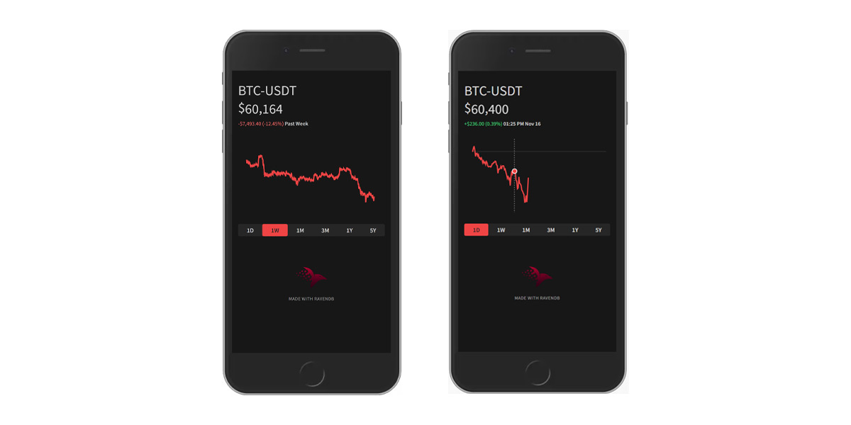
The video above demonstrates a sample crypto price demo modeled after the popular Robinhood trading app. The histogram is powered by RavenDB, a NoSQL document database that offers native support for time series data points.

What is time series data?

A “time series” is usually characterized as data points indexed by time, typically high-frequency in nature. Common sources of time series would be IoT devices, infrastructure, analytics, and stock (or crypto) prices.

What’s so special about it?

At first, you might be thinking, “Could you store these data points within a document database or as rows in a relational database?”

You could but this won’t scale. Storing data like this will quickly devour your storage and it makes your client code do more work to aggregate the data.

Before RavenDB supported time series, a product like InfluxDB would be needed which makes your architecture landscape (and applications) more complex.

Instead, native time series support in RavenDB addresses each of these problems in turn with:

1. Coordinated, atomic transactions across a cluster
2. Rule-based retention policies and storage optimizations
3. Server-side querying and aggregation with indexes

Time series are “extensions” to a document so they benefit from all the infrastructure built around document storage and querying which makes them easier to work with and comes with built-in optimizations.

Working with market data

We’ve built a demo application that showcases time series support in action by tracking the trading price of Bitcoin, inspired by the popular Robinhood trading app.

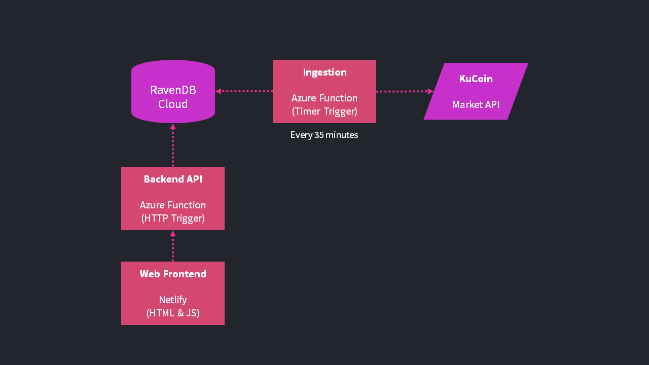
Market data is sourced from KuCoin, a crypto exchange. There are 3 parts to the demo architecture:

• Ingestion: a background job that ingests data from KuCoin into RavenDB
• Backend: an HTTP endpoint that queries the data from RavenDB
• Frontend: a web-based interface that displays the interactive crypto chart

This walkthrough assumes you have some beginner-level knowledge of working with RavenDB and showcases how to work with time series data using the Studio and language SDKs. If you haven’t worked with RavenDB before, the self-guided bootcamp covers all the prerequisites shown here!

Managing time series in RavenDB Studio

We’ll start with looking at how time series works in the Studio interface.

Adding time series to documents

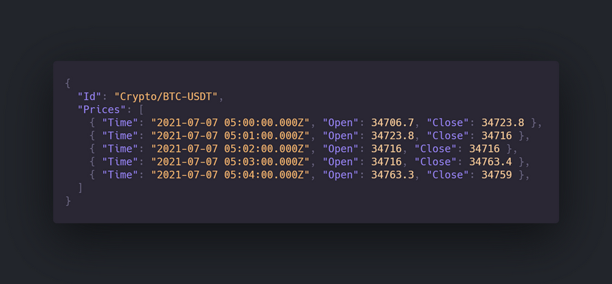
In the sample database, there is a document representing the market symbol for Bitcoin (BTC-USDT):

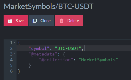
As you can see, there is no time series data in the document itself.

Creating time series collections

Instead, time series can be added through the Studio’s document sidebar:

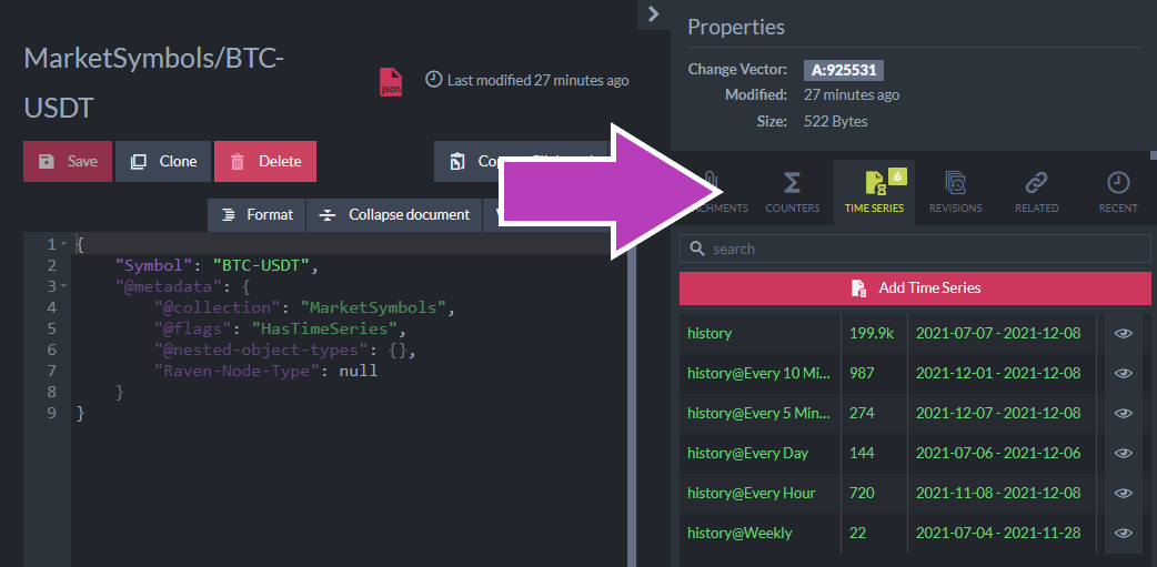
A time series does not exist without values. As soon as you append a value, the time series is “created.” As soon as the last value is deleted, the time series disappears.

Time series entries consist of a series name along with the timestamp and each value:

The first four values are named (Open, Close, High, Low) but the last value is numerically identified as “Value #4.” By default, values are unnamed and are accessed by index but you can optionally configure named values.

Adding named value configuration

Naming values is a best practice as It makes the code clearer and less prone to mistakes.

Within the Studio under Settings and Time Series Configuration, RavenDB provides an interface to manage configuration for time series based on document collection:

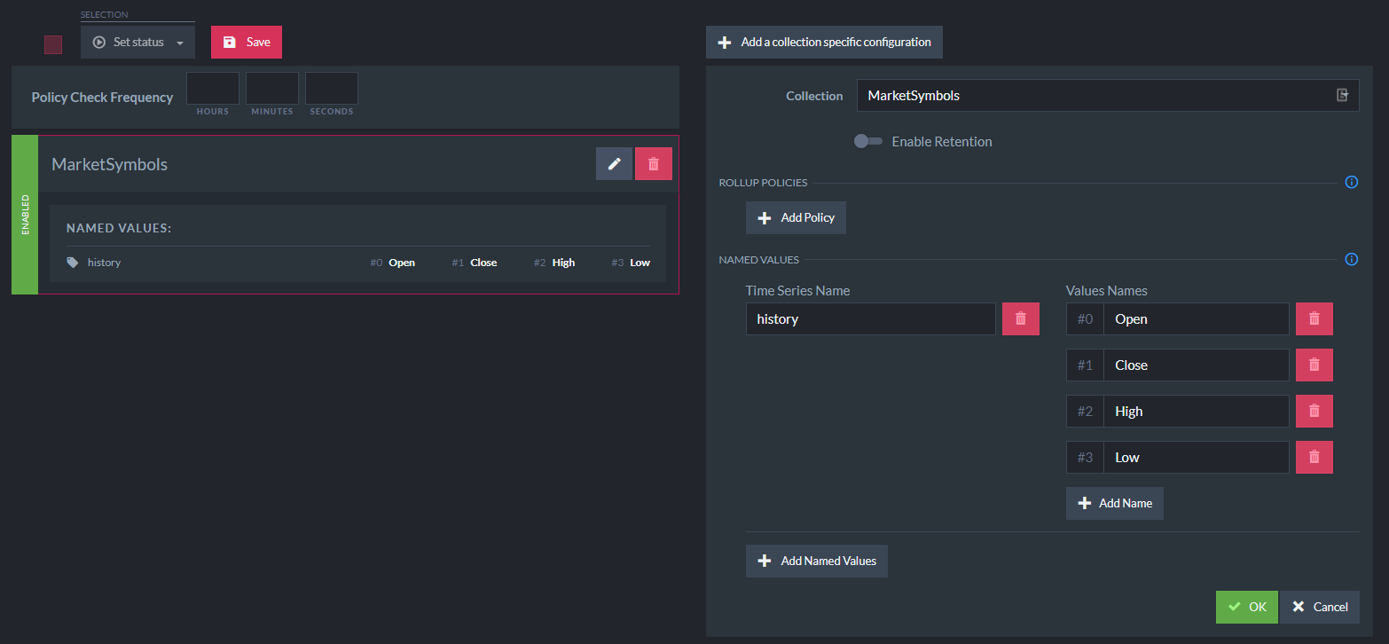
Each name is associated with the value index of the entry and the time series name.

Using time series APIs

Managing time series data in the Studio is a first-class experience but you’ll mostly interact with time series data with code.

Appending and updating time series data

The time series data from the KuCoin API is ingested with a Node.js TypeScript background job hosted in Azure Functions.

Once you open a RavenDB session, the time series APIs operate on documents. First, the Bitcoin document is loaded by ID:

let symbolDoc = await session.load(`MarketSymbols/${marketSymbol}`);

if (!symbolDoc) {
  symbolDoc = {
    symbol: marketSymbol,
    "@metadata": {
      "@collection": "MarketSymbols",
    },
  };
  await session.store(symbolDoc, `MarketSymbols/${marketSymbol}`);
}

Since time series must be associated with a document, we need to create it if it doesn’t exist before we use the timeSeriesFor API.

const timeSeries = session.timeSeriesFor(symbolDoc, "history");

The time series for API takes the entity (document) and name of the time series collection. This does not load any data (yet).

The KuCoin API returns data between two dates as “candlesticks”, visualized like this:

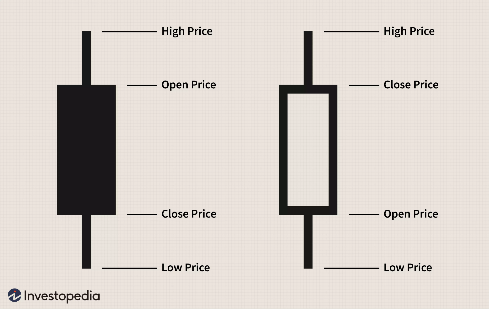
KuCoin represents each candle as a tuple, where each index corresponds to a value of the candle.

The code iterates through the candles and uses array destructuring in TypeScript to take the values and append them to a RavenDB time series:

for (const bucket of buckets) {
  const [
    startTime, 
    openPrice, 
    closePrice, 
    highPrice, 
    lowPrice
  ] = bucket;

  const timestamp = dayjs.unix(startTime);

  timeSeries.append(
    timestamp.toDate(),
    [openPrice, closePrice, highPrice, lowPrice]
  );
}

The append method takes the timestamp (using the dayjs helper library) and the array of values (stored by index).

await session.store(symbolDoc, `MarketSymbols/${marketSymbol}`);
await session.saveChanges();

Like other document-based operations, time series changes are not committed until saveChanges() is called. Time series updates from multiple clients across a cluster do not cause conflicts because RavenDB uses automatic conflict resolution semantics.

Once the background job ingests the data into RavenDB, we can access it and return data to the web frontend to build the histogram.

Eagerly fetching time series

The frontend calls a REST endpoint with query parameters to retrieve a JSON representation and builds the histogram using the Apex Charts library. The backend is written in C# and uses the .NET RavenDB SDK.

When the client requests a market symbol, the code loads the document by ID:

var symbol = await _session.LoadAsync<MarketSymbol>(
  $"MarketSymbols/{marketSymbol}", includes => 
    includes.IncludeTimeSeries("history", 
      from: DateTime.UtcNow.AddDays(-1), to: DateTime.UtcNow));

The IncludeTimeSeries API is used which eagerly fetches the time series data when the document is loaded by RavenDB. This reduces network calls to the database and caches the time series in the session. The from and to arguments allow us to prevent loading the entire data set into memory.

Once the document is loaded, we can use the session TimeSeriesFor API to access the time series:

var historyTimeSeries = _session.TimeSeriesFor<SymbolPrice>(symbol, "history");

Notice we are passing a generic argument with a type of SymbolPrice. This is a struct that strongly types the values.

Adding named value support with classes

I showed you how to manually configure named values in the Studio but we can do the same in code. This allows you to maintain your application code as the source of truth.

Create a struct to name the time series values:

public struct SymbolPrice
{
    [TimeSeriesValue(0)] public double Open;
    [TimeSeriesValue(1)] public double Close;
    [TimeSeriesValue(2)] public double High;
    [TimeSeriesValue(3)] public double Low;
}

TimeSeriesValue takes the index of the value entry to associate with the property.

Now after initializing a DocumentStore, register it with the collection type and series name:

store.Initialize();
store.TimeSeries.Register<MarketSymbol, SymbolPrice>("history");

Note: This feature is only available for statically-typed language SDKs like .NET and Java.

Loading raw time series entries

Once the document is loaded, we can get the latest entries time series by date:

var historyTimeSeries = _session.TimeSeriesFor<SymbolPrice>(symbol, "history");

var latestEntries = await historyTimeSeries.GetAsync(
  from: DateTime.UtcNow.AddDays(-1), to: DateTime.UtcNow);

Without using the IncludeTimeSeries hint, GetAsync would result in an extra network call to the database. Instead, the data is loaded from the session cache.

Document loads are never stale so we can use the latest entry to return the last traded price:

var latestEntry = latestEntries.LastOrDefault();

viewModel.LastUpdated = latestEntry?.Timestamp;
viewModel.LastPrice = latestEntry?.Value.Close ?? 0;

Querying and aggregating time series data

The next step to build the histogram is to aggregate data based on time windows, like “past day” or “past week.”

In a traditional database or application, we would have to load the entire dataset and manually bucket data, which would force us to load all the time series into memory.

In RavenDB, time series data is indexed and can be grouped and filtered on the database server to be returned to the client. This takes advantage of everything else indexes have to offer.

Use the session Query API to query the collection:

var aggregatedHistoryQueryResult = await _session.Query<MarketSymbol>()
  .Where(c => c.Id == symbolId)

Then you can use the helper functions from RavenQuery.TimeSeries to build a time series query expression:

var aggregatedHistoryQueryResult = await _session.Query<MarketSymbol>()
  .Where(c => c.Id == symbolId)
  .Select(c => RavenQuery.TimeSeries<SymbolPrice>(c, "history")
    .Where(s => s.Timestamp > fromDate)
    .GroupBy(groupingAction)
    .Select(g => new
    {
      First = g.First(),
      Last = g.Last(),
      Min = g.Min(),
      Max = g.Max()
    })
    .ToList()
  ).ToListAsync();

There are two variables we are passing in to build the time series query: fromDate and groupingAction.

The fromDate is calculated based on the desired time window the frontend is displaying:

var marketTime = GetMarketTime();
var fromDate = aggregation switch
{
  AggregationView.OneDay => marketTime.LastTradingOpen,
  AggregationView.OneWeek => DateTime.UtcNow.AddDays(-7),
  AggregationView.OneMonth => DateTime.UtcNow.AddMonths(-1),
  AggregationView.ThreeMonths => DateTime.UtcNow.AddMonths(-3),
  AggregationView.OneYear => DateTime.UtcNow.AddYears(-1),
  AggregationView.FiveYears => DateTime.UtcNow.AddYears(-5)
};

The code determines the market open/close schedule (naively) and then can return the appropriate date to filter from for the query.

The groupingAction is ultimately what buckets (groups) the time series data points and is based on what time window is being displayed. The ITimePeriodBuilder API can help build the correct query grouping expression based on simple time units:

Action<ITimePeriodBuilder> groupingAction = aggregation switch
{
  AggregationView.OneDay => builder => builder.Minutes(5),
  AggregationView.OneWeek => builder => builder.Minutes(10),
  AggregationView.OneMonth => builder => builder.Hours(1),
  AggregationView.ThreeMonths => builder => builder.Hours(24),
  AggregationView.OneYear => builder => builder.Hours(24),
  AggregationView.FiveYears => builder => builder.Days(7),
};

This grouping action will tell RavenDB how to bucket the data before returning it by translating it internally to Raven Query Language. This offloads all the processing to the database server.

Once we have the queried data, we build our model and assign the price values for each bucket:

var historyBuckets = new List<MarketSymbolTimeBucket>();
foreach (var seriesAggregation in aggregatedHistory.Results)
{
  historyBuckets.Add(new MarketSymbolTimeBucket()
  {
    Timestamp = seriesAggregation.From,
    OpeningPrice = seriesAggregation.First.Open,
    ClosingPrice = seriesAggregation.Last.Close,
    HighestPrice = seriesAggregation.Max.High,
    LowestPrice = seriesAggregation.Min.Low,
  });
}

Using the named value struct (SymbolPrice), we can access the aggregated values for each pricing bucket. For example, the open price will be the first data point’s Open value in the bucket and the close price is the last data point’s Close value.

This model representation is then returned to the client as JSON and the chart can be built from these data points.

Conclusion

Time series support in RavenDB rivals dedicated products like InfluxDB and there are even more features we didn’t cover in this article such as roll-up policies, tagging, and custom time series indexes.

Want to dive deeper? All of the sample code is available on GitHub in both C# and Node.js form. A sample database is provided which you can import into your RavenDB instance. If you don’t have one, you can create a free one on RavenDB Cloud!

Interested in how RavenDB can handle your time series data needs? We invite you to request a live demo to learn more.