Production deployments

The day you deploy to production can be a very scary day. It is the culmination of months or years of work; the time where you actually get to see the results of your work bearing fruit. Of course, sometimes the fruit is unripe because you pushed the big red button too soon. There is no riskier time in production than just after a new version has been deployed.

I want to recommend the Release It! book by Michael T. Nygard. I read it for the first time over a decade ago, and it made an impact on how I think about production systems. It had a big effect on the design and implementation of RavenDB as well. This chapter will cover topics specific to RavenDB, but you might want to read the Release It! book to understand how to apply some of these patterns to your application as a whole.

There are quite a few concerns that you need to deal with when looking at your deployment plan and strategy. These start with any constraints you have, such as a specific budget or regulatory concerns about the data and how and where you may store it. The good thing about these constraints is that most of the time, they're clearly stated and understood. You also have requirements, such as how responsive the system should be, how many users are expected to use it and what kind of load you have to plan for. Unfortunately, these requirements are often unstated, assumed or kept at such a high enough level that they become meaningless.

You need the numbers

In 2007, I was asked by a client to make sure that the project we were working on would be "as fast as Google." I took him at his word and gave him a quote for 11.5 billion dollars (which was the Google budget for that year). While I didn't get that quote approved, I made my point, and we were able to hammer down what we actually needed from the application.

Giving a quote for $11,509,586,000 is a cry for help. I don't know what "fast" means. That's not how you measure things in a meaningful way. A much better way to state such a request would be to use a similar format to that in Table 15.1.

Reqs / sec	%	Max duration (ms)
100	99%	100
100	99.99%	200
200	99%	150
200	99.9%	250
200	99.99%	350

Table 15.1: SLA table allowing for max response time for requests under different loads

Table 15.1 is actional. It tells us that under a load of 100 requests per second, we should complete 99% of requests in under 100ms and 99.99% requests in under 200ms. If the number of concurrent requests goes up, we also have an SLA set for that. We can measure that and see whether we match the actual requirement.

Developers typically view production as the end of the project. If it's in production, it stays there, and the developers can turn to the next feature or maybe even a different project entirely. The operations team usually has the opposite view. Now that the system's in production, it's their job to babysit it. I don't intend for this to be a discussion of the benefits of having both operations and development insight during the design and development of a system, or even a discussion about closer collaboration in general. You can search for the term "DevOps" and read reams about that.

Instead, I'm going to assume that you are early enough in the process that you can use some of the notions and tools in this chapter to affect how your system is being designed and deployed. If you're farther along, you can start shifting to a point where you match the recommended practices.

And with that, let's dive in and talk about the first thing you need to figure out.

System resources usage

You must have a 386DX, 20MHz or higher processor, 4MB of memory (8MB recommended) and at least 70MB of available hard disk space. Oh, wait. That's wrong. These are actually the system requirements if you want to install Windows 95.

I want to refer you back to Table 15.1. Before you can make any decisions, you need to know what kind of requirements are going to be placed on your system. Is this a user-facing system or B2B? How much data will it need to handle? How many requests are expected? Are there different types of requests? This is important enough concept that it's worth repeating. There are a lot of good materials about how to go about your system's requirements; I'll point you again to the Release It! book for more details.

There is an obvious correlation between the load on your system and the resources it consumes to handle this load. Figure 15.1 shows a couple of graphs from a production system. This isn't peak load, but it isn't idle either.¹

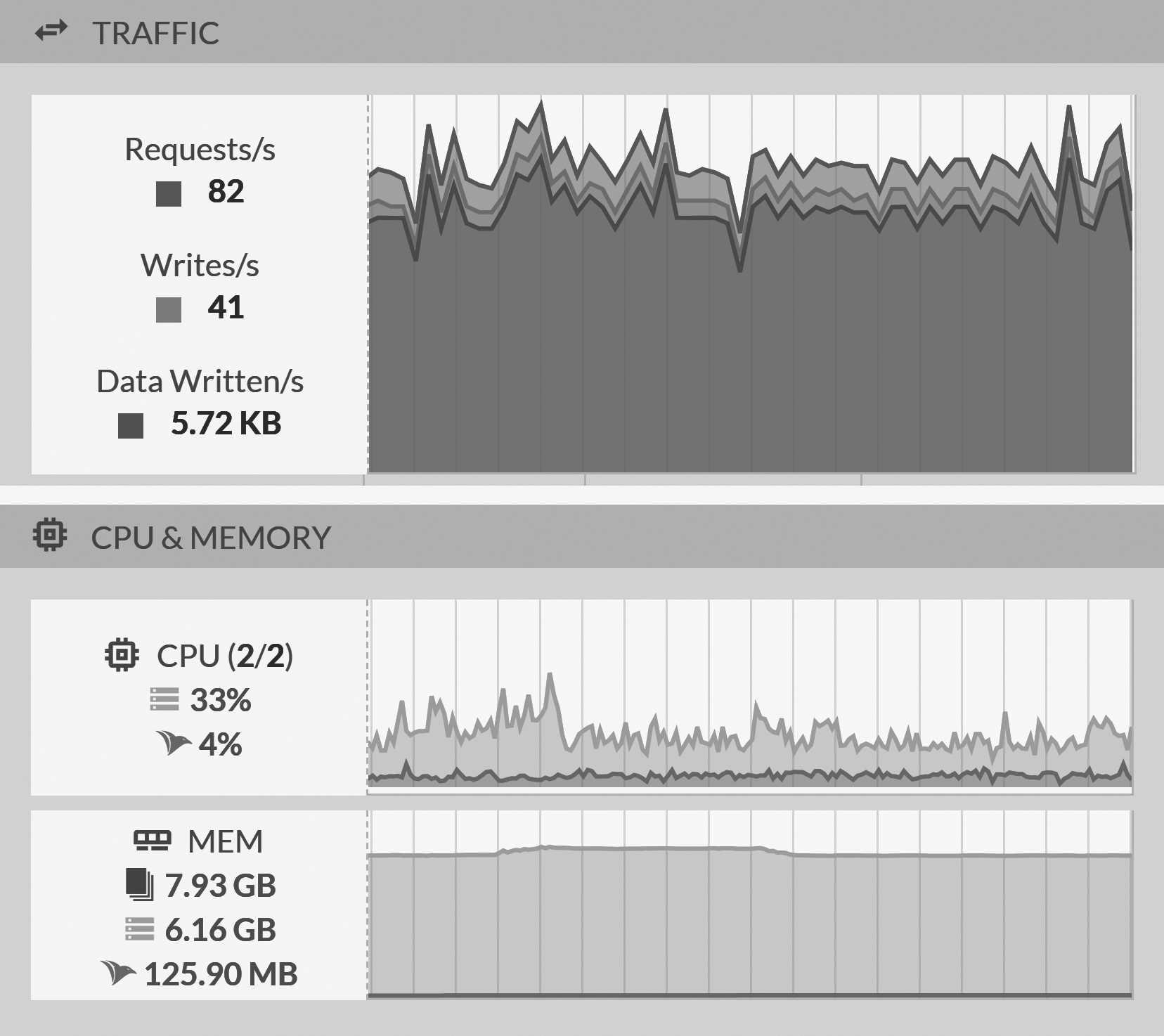
This particular machine is running on an Amazon EC2 t2.large instance with 2 cores and 8 GB of memory. The machine isn't particularly loaded, with enough spare capacity to handle peaks of three to four times as many requests per second. Of course, this is just a very coarse view of what is going on, since it is missing the request latencies. We can get that information as well, as you can see in Figure 15.2. (In the Studio go to Manage Server and then Traffic Watch).

Things seems to be fine: the average request time is low, and even the maximum isn't too bad. We can dive into percentiles and metrics and all sort of details, but at this point getting too specific won't be of much relevance for this book.

If you're already in production, the RavenDB Studio has already surfaced these numbers for you, which means that you can act upon them. For one thing, the correlation between the requests on the server and the load on the server can be clearly seen in Figure 15.1, and that can help you figure out what kind of system you want to run this on.

Given that you are not likely to have an infinite budget, let's go over how RavenDB uses the machine's resources and what kind of impact that is likely to have on your system.

Disk

By far the most important factor affecting RavenDB performance is the disk. RavenDB is an ACID database, which means that it will not acknowledge a write until it has been properly sent to the disk and confirmed to be stored in a persistent manner. A slow disk can make RavenDB wait for quite a while until it has disk confirmation, and that will slow down writes.

RavenDB is quite proactive in this manner and will parallelize writes whenever possible, but there is a limit to how much we can play with the hardware. At the end of the day, the disk is the final arbiter of when RavenDB can actually declare a transaction successful.

If you are using physical drives, then the order of preference at this time is to use NVMe if you can. Failing that, use a good SSD. Only if you can't get these (and you should), go for a high-end HDD. Running a production database load on a typical HDD is not recommended. It's possible, but you'll likely see high latencies and contention in writing to the disk, which may impact operations. This strongly relates to your actual write load.

What kind of request are you?

It's easy to lump everything into a single value — requests per second — but not all requests are made equal. Some requests ask to load a document by id (cheap), others may involve big projections over a result set containing dozens of documents (expensive). Some requests are writes, which will have to wait for the disk, and some are reads, which can be infinitely parallel.

When doing capacity planning, it's important to try to split the different types of requests so we can estimate what kind of resource usage they're going to need. In Figure 15.1, you can see that RavenDB divides requests into the total number (Requests/s) and then the number of writes out of that total. This gives us a good indication of the split in requests and the relative costs associated with such requests.

If you're using network or cloud disks, be sure to provision enough IOPS for the database to run. In particular, when using a SAN, do not deploy a cluster where all the nodes use the same SAN. This can lead to trouble. Even though the SAN may have high capacity, under load, all nodes will be writing to it and will compete for the same resources. Effectively, this will turn into a denial of service attack against your SAN. The write load for RavenDB is distributed among the nodes in the cluster. Each node writes its own copy of the data, but all data ends up in the same place.

I strongly recommend that when you deploy a RavenDB cluster, you use independent disks and I/O channels. RavenDB assumes that each node is independent of the others and that the load one node generates shouldn't impact operations on another.

You might have noticed that so far I was talking about the disk and its impact on writes, but didn't mention reads at all. This is because RavenDB uses memory-mapped I/O, so reads are usually served from the system memory directly.

Memory

The general principle of memory with RavenDB is that the more memory you have, the better everything is. In the ideal case, your entire database can fit in memory, which means that the only time that RavenDB will need to go to disk is when it ensures a write is fully persisted. In more realistic scenarios, when you have a database that is larger than your memory, RavenDB will try to keep as much of the database as you are actively using in memory.

In addition to memory-mapped files, RavenDB also uses memory for internal operations. This can be divided into managed memory (that goes through the .NET GC) and unmanaged memory (that is managed by RavenDB directly). Typically, the amount of memory being allocated will only be large if RavenDB is busy doing heavy indexing, such as when rebuilding an index from scratch.

For good performance and stability, it's important to ensure that the working set of RavenDB (the amount of data that is routinely accessed and operated on at any given time) is less than the total memory on the machine. Under low memory conditions, RavenDB will start scaling down operations and use a more conservative strategy for many internal operations in an attempt to reduce the memory pressure.

If you are running on a machine with a non-uniform memory access (NUMA) node, that can cause issues. RavenDB doesn't use NUMA-aware addressing for requests or operations, which can cause memory to jump between NUMA nodes, as well as high CPU usage and increased latencies. We recommend that you configure the machine to behave in a non-NUMA-aware fashion. Alternatively, you could run multiple instances of RavenDB on the machine, each bound to a specific NUMA node.

CPU

Given an unlimited budget, I want the fastest CPU with the most cores. Reads in RavenDB scale linearly with the number of cores that a machine has, but sequential operations such as JSON parsing are usually bounded by the speed of the individual cores.

RavenDB makes heavy use of async operations internally to reduce the overall number of context switches. But the decision to prioritize more cores over faster cores is one you have to make based on your requirements. More cores means that RavenDB can have a higher concurrent number of requests, but will also have higher latency. Fewer and faster cores means faster responses, but also fewer concurrent requests.

The choice between faster cores or more cores is largely academic in nature. RavenDB is a very efficient database. We have tested RavenDB with a Raspberry Pi 3, a $25 computer that uses a quad-core 1.2GHz ARM CPU and 1GB of RAM. On that machine, we were able to process a little over 13,000 document reads per second. Those were simple document loads without complex queries or projections, but that should still give you some idea about the expected performance of your production systems.

Network

As you can imagine, network usage in RavenDB is important. With enough load, RavenDB can saturate a 10GB connection, sending out gigabytes of data per second. But if you get to this point, I suggest taking a look at your application to see what it's doing. Very often, such network saturation is the result of the application asking for much more data than is required.

A good example is wanting to load the list of orders for a customer and needing to show a grid of the date, total order value and the status of the order. In some cases, the application will pull the full documents from the server, even though it uses only a small amount of the data from them. Changing the application to project only the relevant information is usually a better overall strategy than plugging in a 20GB card.

An important consideration for network usage is that RavenDB will not compress the outgoing data by default when using HTTPS. If you are talking to RavenDB from a nearby machine (same rack in the data center), there is usually enough network capacity that RavenDB can avoid spending time compressing the responses. There is also the BREACH attack for compressed HTTPS to consider, which is why automatic compression is off by default.

Compression on the wire is controlled via Http.UseResponseCompression and Http.AllowResponseCompressionOverHttps settings. You can also control the compression level using the Http.GzipResponseCompressionLevel setting, favoring speed over compression rate or vice versa. On a local network, it is probably best to not enable that; the CPU's time is better spent handling requests, not compressing responses.

Common cluster topologies

RavenDB is quite flexible in the ways it allows you to set itself up for production. In this section, we are going to look at a few common configuration topologies for RavenDB, giving you the option to pick and chose what is best for your environment and needs. These aren't the only options, and you can usually mix and match them.

A RavenDB cluster and what it's good for

A cluster in RavenDB is a group of machines that is managed as a single unit. A cluster can contain any number of databases that are spread across its nodes. Each database can have multiple copies which are are replicated to some (or all) of the nodes, depending on the replication factor for the specific database.

RavenDB doesn't split the database data among the various nodes, but replicates all the data in the database to each of the nodes in the database group.²

You'll typically use a dedicated database per application, potentially with some data flows (ETL and external replication) between them. These databases are hosted on a single cluster, which simplifies management and operations. Let's see how we actually deploy RavenDB in various scenarios and the pros and cons of each option.

A single node

The single node option is the simplest one. Just have one single node and run everything on top of that. You can see an example of this topology in Figure 15.3.

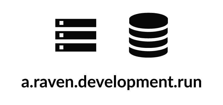
In this mode, all the databases you use are on the same node. Note that this can change over time. Any RavenDB node is always part of a cluster. It may be a cluster that only contains itself, but it is still a cluster. In operational terms, this means that you can expand this cluster at any point by adding more nodes to it and then decide how to arrange the databases on the cluster.

This mode is popular for development, UAT, CI and other such systems. While possible, it is not recommended that you use a single node configuration for production because it has a single point of failure. If this single node is down, there is no one else around that can take its duties, and that makes any issues with the node high priority by definition.

The better alternative by far is a proper cluster.

The classic cluster

The classic cluster has either three or five nodes. The databases are spread across the cluster, typically with a replication factor of two or three. Figure 15.4 shows a three-node cluster where the 'Helpdesk' and 'Users' databases have a replication factor of three, while 'Fulfillment', 'Ledger' and 'Orders' databases have a replication factor of two.

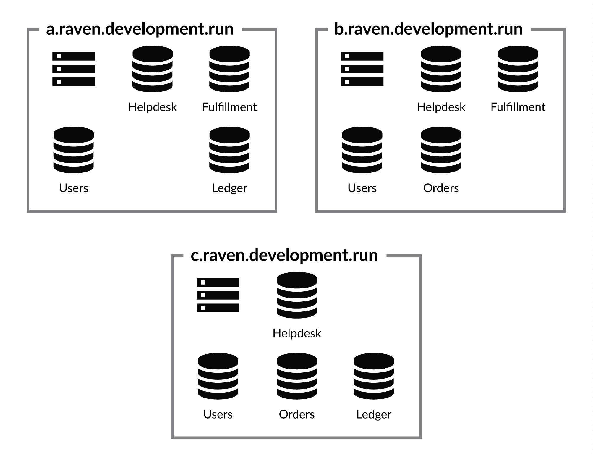
In the three-node cluster mode shown in Figure 15.4, we know that we can lose any node in the cluster and have no issue continuing operations as normal. This is because at the cluster level, we have a majority (2 out of 3) and we are guaranteed to have all the databases available as well.

In this way, we've reduced the density from five databases per server to four. Not a huge reduction, but it means that we have more resource available for each database, and with that we've gained higher security.

You don't need a majority

The topologies shown in Figure 15.4 and Figure 15.5 showcase a deployment method that ensures that as long as a majority of the nodes are up, there will be no interruption of service. This is pretty common with distributed systems, but it isn't actually required for RavenDB.

Cluster-wide operations (such as creating and deleting databases, assigning tasks to nodes in the cluster or creating indexes) require a majority to be accessible. But these tend to be rare operations. The most common operations are the reads and writes to documents, and these can operate quite nicely even with just a single surviving node. The mesh replication between the different databases uses a gossip protocol (discussed in more depth in Chapter 6) with a multi-master architecture.

All reads and writes can go to any database in the database group and they will be accepted and processed normally. This gives the operations team a bit more freedom with how they design the system and the ability to choose how much of a safety margin is needed compared to the resources required.

Another classic setup is the five-node cluster, as shown in Figure 15.5. Each node in the cluster contains three databases and the cluster can survive up to two nodes being down with no interruption in service. At this point, you need to consider whether you actually need this level of redundancy.

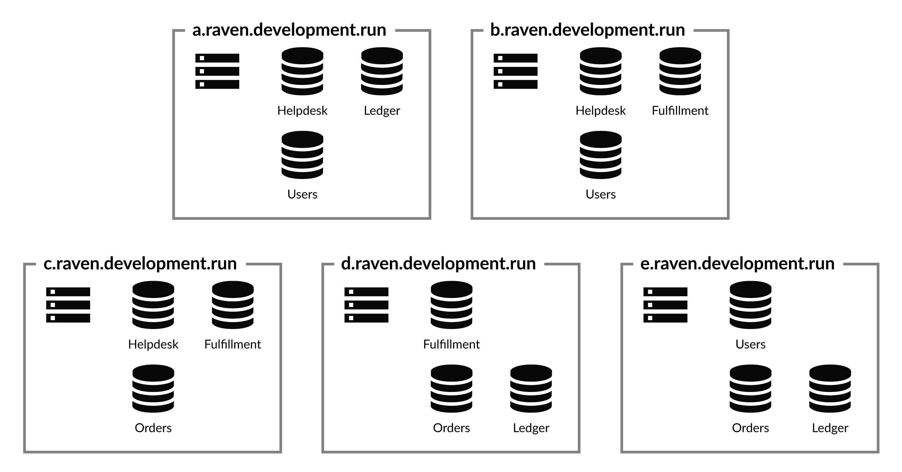
There are many cases where you can live with a lower redundancy level than the one shown in Figure 15.5. Having a five-node cluster with each of the databases having a replication factor of two is also an option. Of course, in this mode, losing two specific nodes in the cluster may mean that you'll lose access to a particular database. What happens exactly depends on your specific failure. If you lose two nodes immediately, the database will become inaccessible.

If there is enough time between the two nodes failures for the cluster to react, it will spread the database whose node went down to other nodes in the cluster to maintain the replication factor. This ensures that a second node failure will not make a database inaccessible.

High availability clusters

RavenDB clusters and their highly available properties were discussed at length in Chapters 6 and 7. Here it is important to remember that the cluster will automatically work around a failed node, redirecting clients to another node, re-assigning its tasks and starting active monitoring for its health.

If the node is down for long enough, the cluster may decide to add extra copies of the databases that resided on the failed node to ensure the proper number of replicas is kept, according to the configured replication factor.

This particular feature is nice when you have a five-node cluster, but most times you'll use a replication factor of three and not have to think about the cluster moving databases around. This is far more likely to be a consideration when the number of nodes you have in the cluster grows much higher.

Some nodes are more equal than others

RavenDB uses a consensus protocol to manage the cluster. This means that any cluster-wide operation requires acknowledgment from a majority of the nodes in the cluster. For a five-node cluster, this means that each decision requires the leader's confirmation as well as the confirmation of two other nodes to be accepted. As the size of the cluster grows, so does the size of the majority. For example, with a seven–node cluster, you need a majority of four.

Because of this, you typically won't increase the size of your cluster whenever you need more capacity. If you have enough databases and load to need a 20-node cluster, each decision will require 11 confirmations. That... is quite high. Instead, we arrange the cluster in two ranks.

In the first rank, we have the cluster members. These are nodes that can vote and become the cluster leader. You'll typically have three, five or seven of them, but no more than that. The higher the number of member nodes, the more redundancy you'll have in the cluster. But what about the rest of the cluster nodes?

The rest of the cluster nodes aren't going to be full members. Instead, they are marked as watchers in the cluster. You can see how this topology looks like in Figure 15.6.

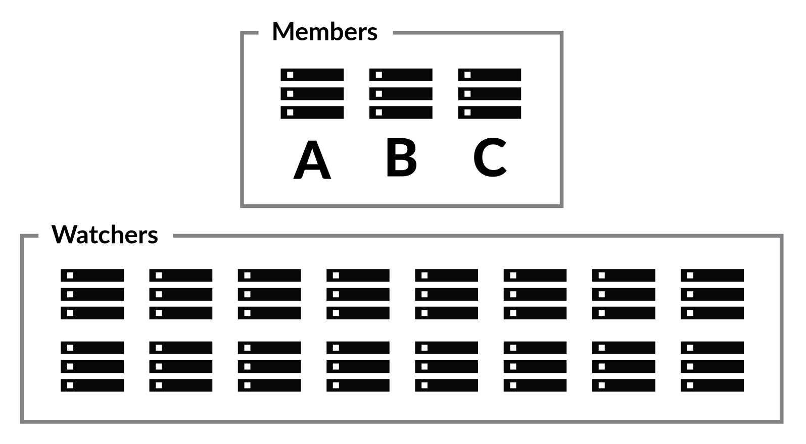
A watcher in the cluster is a fully fledged cluster node. The node hosts databases and is managed by the cluster, just like any other node. However, it cannot be voted as the leader, and while it is informed about any cluster decision, the cluster doesn't count a watcher's vote towards the majority. A cluster majority is always computed as: floor(MembersCount / 2) + 1, disregarding the watchers (which are just silent observers).

A watcher node can be promoted to a member node (and vice versa), so the decision to mark a node as a member or watcher doesn't have long-term implications. If a member node is down and you want to maintain the same number of active members, you can promote a watcher to be a member. But keep in mind that promoting a node is a cluster operation that requires a majority confirmation among the cluster members, so you can't promote a node if the majority of the members is down.

Primary/secondary mode

The primary/secondary topology is a common topology to achieve high availability. A good example of this topology can be seen in Figure 15.7. You have a primary server that does all the work and a secondary server that replicates the data. This is also called active/passive topology.

With RavenDB, using a two-node cluster is not a good idea. The majority of two is still two, after all, so even a single node failure will make the cluster unavailable.³ A two-node cluster is sometimes chosen as the selected topology when you want to manually control failover behavior for some reason. We'll cover this option in the next section.

Database group topologies

We've talked about the topology of the cluster, but most of the work done with RavenDB is at the database level. Let's zoom in to see how we should deploy our databases in production.

Reminder: database groups and database instances

A database group is the set of nodes that holds the individual instances of the database. Each one of the database instances will replicate all its data to any of its sibling instances on the other nodes in the database group.

The database group as a whole is being managed by the cluster: assigning tasks to various nodes in the group, determining the nodes' priority order for clients, etc. At the same time, each instance constantly gossips with other members of the group, sharing new and updated information and reconciling any changes that have happened in the meantime.

This gossip is done independently from the cluster behavior and continues even under error conditions that cause the cluster to become inoperable. Clients know the database group topology and will try another node if the node they tried talking to isn't responding. This leads to a robust system in which the cluster, the database group members and the clients are all working together to achieve maximum uptime.

There a few considerations to take into account about the database topology. First, we need to decide the appropriate replication factor for the database. The more copies of the data we have, the safer we are against catastrophe. On the other hand, at some point, we are safe enough and increasing the replication factor any further is just burning through disk space.

Second, we need to consider what kind of access pattern the client should use. By default, clients will access the database instances in a database group in the order they are defined on the server. You can see that in Figure 15.8 and on the Studio under Settings and then Manage Database Group.

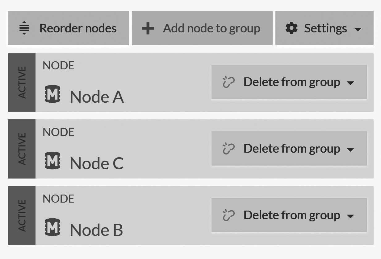
As you can see in Figure 15.8, the admin can control this order. This is designed not just to comply with some people's OCD tendencies — no, I'll not call it CDO, even though that is the proper way to alphabetize it — the order of nodes in this list matters. This list forms the nodes' priority order by which the clients will access a database instance by default.

If a client cannot talk to the first node in the list, it will try the second, etc. Reordering the nodes will cause the server to inform the clients about the new topology for the next requests they make.

Aside from the operations team manually routing traffic, there is also the cluster itself that can decide to change the order of nodes based on its own cognizance, to handle failures, to distribute load in the cluster, etc. You can also ask clients to use a round robin strategy (configured via Settings, Client Configuration and then selected from the Read balance behavior dropdown) in order to spread the read load among the nodes.

In addition to defining a database group inside a single cluster, you also have the option of connecting databases from different clusters. This can be done in a one–way or bidirectional manner.

Using replication outside the cluster

Database groups have fairly rigid structures. Except for determining which nodes the databases reside on, you can't configure much on a per-node basis. Sometimes, you want to go beyond that. Maybe you want different indexes on different nodes, or to have a "firebreak" type of failover where only if you manually switch things over will clients fail over to a secondary node. Or maybe you just need a higher degree of control in general.

At that point, you will no longer use the cluster to manage things; you'll take the reins yourself. You'll do this by manually defining the data flow between databases using external replication. We covered external replication in Chapter 7. Using external replication, you can control exactly where and how the data will travel. You aren't limited to just defining the data flow between different database instances in the same cluster.

When using external replication, you need to remember:

• Clients will not follow external replication in the case of failure.
• Indexes are not replicated via external replication.
• The configuration and settings between the nodes can be different (this impacts things like expiration, revisions, etc.).
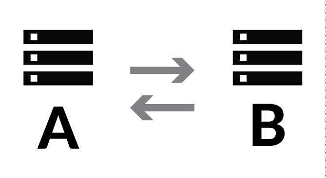
• External replication is unidirectional. If you want to have documents flowing both ways, you'll have to define the replication from both ends.
• External replication is a database group-wide task that is managed by the cluster with automatic failure handling and failover on both source and destination.

These properties of external replication open up several interesting deployment options for your operations team. Probably the most obvious option is offsite replicas. An offsite replica can be used as part of your disaster recovery plans so that you have a totally separate copy of the data that isn't directly accessed from anywhere else.

This is also where the delayed replication feature comes into play. Configuring a delay into external replication gives you time to react in case something bad happens to your database (such as when you've run an update command without using a where clause).

The fact that external replication is a database group-wide operation and that its target is a database group in another RavenDB cluster (not a single node) is also very important. Consider the topology in Figure 15.9.

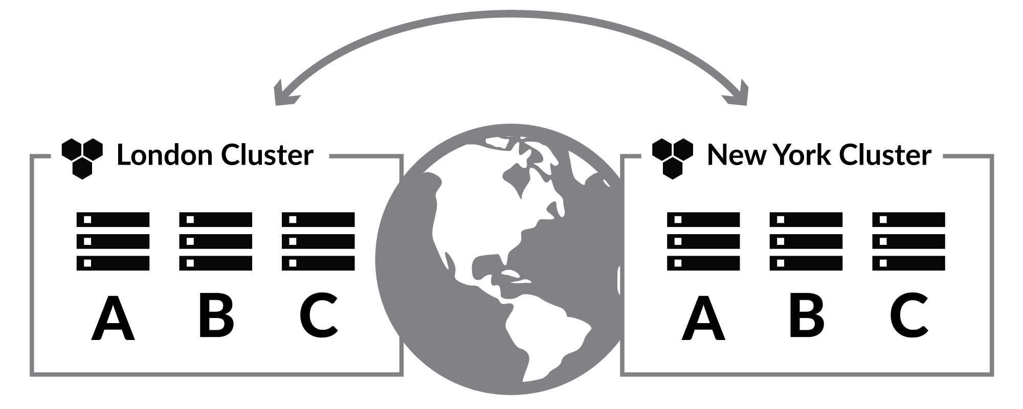
In Figure 15.9, you have two independent clusters deployed to different parts of the world. These clusters are connected via bidirectional external replication. Any change that happens on one of these clusters will be reflected in the other. Your application, on the other hand, is configured to use the cluster in the same data center as the application itself. There is no cross-data center failover happening here. But the data is fully shared.

This is a good way to ensure high availability within the same data center, global availability with a geo-distributed system and good locality for all data access since the application will only talk to its own local nodes. In this case, we rely on the fact that clients will not fail over across external replication. This way if we lose a whole data center, we'll simply route traffic from your application to the surviving data center rather than try to connect from one data center to another for all our database calls.

Ideal number of databases per node

It's rare that you'll only have a single database inside your cluster. Typically, you'll have each application using its own database. Even inside a single application, there are many good reasons for having separate pieces store information separately. This leads to an obvious question: how many databases can we squeeze onto each node?

There is no generic answer to this question. But we can break down what RavenDB does with each database and then see how much load that will take. Each database that RavenDB hosts uses resources that can be broken up into memory, disk and threads. It might seem obvious, but it's worth repeating: the more databases you have on a single node, the more disk space you're using. If all these databases are active at once, they are going to use memory.

I've seen customers packing 800-900 databases into a single server, who were then surprised to find that the server was struggling to manage. Sure, each of those databases was quite small, 1-5GB in size, but when clients started to access all of them, the database server was consuming a lot of resources and often failed to keep up with the demand. A good rule of thumb is that it's better to have fewer, larger databases than many small databases.

Each database holds a set of resources with dedicated threads to apply transactions, run indexes, replicate data to other instances, etc. All of that requires CPU, memory, time and I/O. RavenDB can do quite nicely with a decent number of databases on a single node, but do try to avoid packing them too tightly.

A better alternative if you have a lot of databases is to simply break the node into multiple nodes and spread the load across the cluster. This way, your databases aren't all competing for the same resources, which makes it much easier to manage things.

Increasing the database group capacity

A database group is not just used for keeping extra copies of your data, although that is certainly nice. Database groups can also distribute the load on the system at large. There are many tasks that can be done at the database group level. We've already looked at how Read balance behavior shares the query load between the nodes, but that's just the beginning.

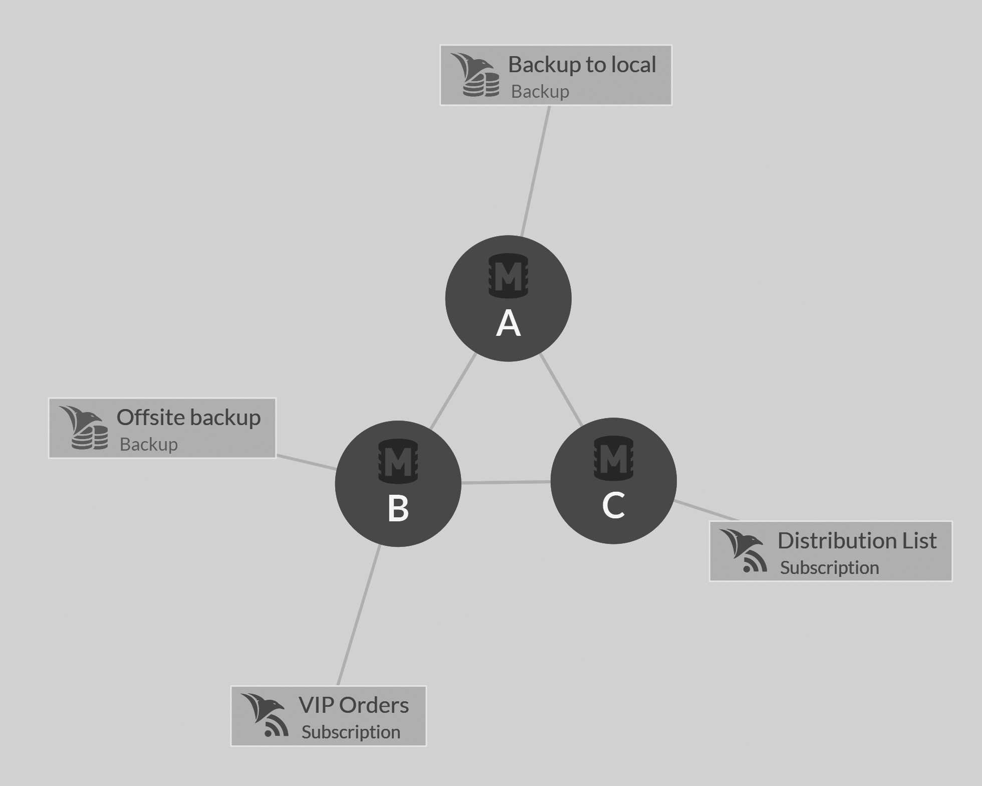
Subscriptions, ETL processes, backups and external replication are all tasks that the cluster will distribute around the database group. You can also define such tasks to be sticky so they'll always reside on the same node. The idea is that you can distribute the load among all the instances you have. You can see how that works in Figure 15.10.

If needed, you can increase the number of nodes a database group resides on, giving you more resource to distribute among the various tasks that the database group is responsible for. This can be done via the Settings, Manage Database Group page by clicking on Add node to group and selecting an available node from the cluster. This will cause RavenDB to create the database in the new node in a promotable state. The cluster will assign one of the existing nodes as the mentor, replicating the current database state to the new database.

Once the new database is all caught up (which for large databases can take a bit of time) the cluster will promote the node to a normal member and redistribute the tasks in the database group in a fair manner. You need to be aware that for the duration of the expansion, the mentor node is going to be busier than usual. Normally, it's not busy enough to impact operations, but you still probably don't want to be doing it if your cluster is at absolute full capacity.

Databases, drives and directories

I already talked about the importance of good I/O for RavenDB earlier in this chapter. That was in the context of deploying a cluster; now I want to focus on the I/O behavior of a single node and even a single database inside that node.

Using a database's data directory as the base, RavenDB uses the format shown in Listing 15.1.

Listing 15.1 On disk structure of the Northwind database folder in RavenDB

*-- Indexes
| *-- Orders_ByCompany
| | *-- Journals
| | | *-- 0000000000000000001.journal
| | *- Raven.voron
| *-- Orders_Totals
| | *-- Journals
| | | *-- 0000000000000000001.journal
| | | *-- 0000000000000000002.journal
| | *-- Raven.voron
| *-- Product_Search
| *-- Journals
| | *-- 0000000000000000002.journal
| *-- Raven.voron
*-- Journals
| *-- 0000000000000000003.journal
| *-- 0000000000000000004.journal
*-- Raven.voron

You can see that the most important details are Raven.voron (the root data file), Journals (where the transaction write ahead journals live) and Indexes (where the indexes details are kept). Interestingly, you can also see that the Indexes structure actually mimics the structure of the database as a whole. RavenDB uses Voron to store the database itself and its indexes (in separate locations).

This is done intentionally because it gives the operations team the chance to play some interesting games. This split allows you to define where the data will actually reside. It doesn't have to all sit on the same drive. In fact, for high-end systems, it probably shouldn't.

Using the operating system tools

Splitting data and journals into separate physical devices gives us better concurrency and helps us avoid traffic jams at the storage level.

Instead of having to configure separate paths for journals, data and indexes, RavenDB relies on the operating system to handle all that. On Linux, you can use soft links or mount points to get RavenDB to write to a particular device or path. On Windows, junction points and mount points serve the same purpose.

The Journals directory files are typically only ever written to. This is done in a sequential manner, and there is only ever a single write pending at any given time. Journals always use unbuffered writes and direct I/O to ensure that the write bypasses all caches and writes directly to the underlying drive. This is important when making sure that the transaction is properly persisted. It's also in the hot path for a transaction commit, since we can't confirm that the transaction has actually been committed until the disk has acknowledged it.

The Raven.voron file is written to in a random manner, typically using memory-mapped I/O. Occasionally an fsync is called on it. These writes to the memory-mapped file and the fsync are not in the hot path of any operation, but if they're too slow, they can cause RavenDB to use memory to hold the modified data in the file while waiting for it to sync to disk. In particular, after a large set of writes, fsync can swamp the I/O on the drive, slowing down other operations (such as journal writes).

Each of the directories inside the Indexes directory holds a single index, and the same rules about Raven.voron and Journals apply to those as well, with the exception that each of them is operating independently and concurrently with the others. This means that there may be many concurrent writes to the disk (either for the indexes' Journals or for the writes to the Raven.voron files for the indexes).

You can use this knowledge to move the Indexes to a separate drive to avoid congesting the drive that the database is writing to. You can also have the Journals use a separate drive, maybe one that is set up to be optimal for the kind of access the journals have.

The idea is that you'll split the I/O work between different drives, having journals, indexes and the main data file all on separate physical hardware. In so doing, you'll avoid having them fighting each other for I/O access.

Paths in the clusters

In a cluster, you'll often use machines that are identical to one another. That means that paths, drives and setup configurations are identical. This makes it easier to work in the cluster because you don't have to worry about the difference between nodes. There's nothing in RavenDB that actually demands this; you can have a database node with a drive D: running Windows and another couple running Ubuntu with different mount point configurations, all in the same cluster.

However, when you need to define paths in the cluster, you should take into account that whatever path you define is not only applicable for the current node, but may be used on any node in the cluster. For that reason, if you define an absolute path, choose one that is valid on all nodes.

For relative paths, RavenDB uses the DataDir configuration value to determine the base directory from which it will start computing. In general, I would recommend using only relative paths, since this simplifies management in most cases.

Network and firewall considerations

RavenDB doesn't require much from the network in order to operate successfully. All the nodes need to be able to talk to each other; this refers to both the HTTPS port used for external communication and the TCP port that is mostly used for internal communication. These are configured via ServerUrl and ServerUrl.Tcp configuration options, respectively.

If you don't have to worry about firewall configurations, you can skip setting the ServerUrl.Tcp value, in which case RavenDB will use a random port (the nodes negotiate how to connect to each other using the HTTPS channel first, so this is fine as long as nothing blocks the connection). But for production settings, I would strongly recommend setting a specific port and configuring things properly. At some point, there will be a firewall, and you don't want to chase things.

Most of the communication to the outside world is done via HTTPS, but RavenDB also does a fair bit of server-to-server communication over a dedicated TCP channel. This can be between different members of the same cluster, external replication between different clusters or even subscription connections from clients. As discussed in Chapter 13, all communication channels used when RavenDB is running in a secured mode are using TLS 1.2 to secure the traffic.

RavenDB will also connect to api.ravendb.net to get notifications about version updates and check the support and licensing statuses. During setup and certificate renewal, we'll also contact api.ravendb.net to manage the automatic certificate generation if you're using RavenDB's Let's Encrypt integration (see Chapter 13). For these reasons, you should ensure that your firewall is configured to allow outgoing connections to this URL.

In many cases, using certificates will check the Authority Information Access (AIA) and Certification Revocation List (CRL). This is usually controlled by system-level configuration and security policies and is basically a way to ensure trust in all levels of the certificate. These checks are usually done over HTTP (not HTTPS), and failing to allow them through the firewall can cause slow connections or failure to connect.

Configuring the operating system

I want to point out a few of the more common configuration options and their impacts on production deployments. The online documentation has full details on all different options you might want to play with.

On Linux, the number of open file descriptors can often be a stumbling block. RavenDB doesn't actually use that many file descriptors.⁴ However, network connections are also using file descriptors, and under load, it's easy to run out of them. You can configure this with ulimit -n 10000.

Another common issue on Linux is wanting to bind to a port that is lower than 1024 (such as 443 for HTTPS). In cases like this, since we want to avoid running as root, you'll need to use setcap to allow RavenDB to listen to the port. This can be done using sudo setcap CAP_NET_BIND_SERVICE=+eip /path/to/Raven.Server.

When using encryption, you may need to increase the amount of memory that RavenDB is allowed to lock into memory. On Linux, this is handled via /etc/security/limits.conf and increasing the memlock values. For Windows, you may need to give the RavenDB user the right to Lock pages in memory.

Summary

We started this chapter talking about capacity planning and, most importantly, measurable SLAs, without which operations teams resort to hand waving, imprecise language and the over-provisioning of resources. It's important to get as precise an idea as possible of what your system is expected to handle and in what manner. Once you have these numbers, you can plan the best way to actually deploy your system.

We went over the kinds of resources RavenDB uses and how we should evaluate and provision for them. We took a very brief look at the kinds of details we'll need for production. We talked about the kinds of disks on which you should run RavenDB (and the kind you should not). I/O is very important for RavenDB, and we'll go back to this topic in the next chapter as well. We covered how RavenDB uses memory, CPU and the network. In particular, we went over some of the settings (such as HTTP compression) that are only really meaningful for production.

We then talked about different cluster topologies and what they are good for. We looked at the single-node setup that is mostly suitable for development (and not suitable for production) and highly available clusters that can handle node failures without requiring any outside involvement. We went over the considerations for replication factors in our cluster, which depend on the value of the data, how much extra disk space we can afford and the results of being offline.

We then talked about large clusters composed of many nodes in tiers. We covered members nodes that form the "ruling council" of the cluster and can vote on decisions and become the leader, as well as the watcher nodes (the "plebs") that cannot vote but are still being managed by the cluster. Separating clusters into member and watcher nodes is a typical configuration when you have a very large number of databases and want to scale out the number of resources that will be used.

We then narrowed our focus to the database level, talking about database group topologies and how they relate to the behavior of the system in production. As an administrator of a RavenDB system, you can use database topology to dictate which node the clients will prefer to talk to, whether they will use a single node or spread their load across multiple nodes and how tasks should be assigned within the group.

Beyond the database group, you can also use external replication to bridge different databases, including databases in different clusters. We looked at an example that shared data between London and New York data centers in two separate clusters. The option to bridge databases in different clusters gives you better control over exactly how clients will behave if an entire data center goes down.

We then talked about the number of databases we want to have per node. RavenDB can support a decent number of databases without issue, but in general, we prefer fewer and larger databases over more and smaller. We also looked into what is involved in expanding the database group and adding more nodes (and capacity) to the database.

Following that, we dove into how RavenDB stores data on disk and what access patterns are used. You can use this information during deployment to split the data, indexes and the journals to separate physical drives, resulting in lower contentions on the I/O devices and giving you higher overall performance.

We ended the chapter by discussing some of the minor details involved in deploying to production, the kinds of firewall and network settings to watch out for and the configuration changes we should make to the operating system.

This chapter is meant to give you a broad overview of deploying RavenDB, and I recommend following it up by going over the detailed instructions in the online documentation. Now that your RavenDB cluster is up and running, you need to know how to maintain it. Next topic: monitoring, troubleshooting and disaster recovery.