Querying in RavenDB

Queries in RavenDB use a SQL-like language called "RavenDB Query Language,"¹ henceforth known as RQL.²

You've already run into the RavenDB Query Language when using subscriptions, even if I didn't explicitly call it out as such. Both subscriptions and queries use RQL, although there are a few differences between the two supported options. The idea with RQL is to directly expose the inner workings of the RavenDB query pipeline in a way that won't overwhelm users.

If you're interested in a simple listing of query capabilities and how to do certain queries, head over to the online documentation, where all of that information is found. I find it incredibly boring to list all that stuff. So instead, we'll cover the material by examining it in a way that gives you insight into not only how to query RavenDB but also what RavenDB actually needs to do to answer the query.

Where is the code?

This chapter is going to focus solely on the query behavior of RavenDB. As such, we'll be working in the Studio, generating queries and looking at documents. We'll look at code to consume such queries from the client API in later chapters.

Here, we'll first take a brief look at how RavenDB is processing queries. Then we'll get started on actually running queries. We'll start from the simplest scenarios and explore all the nooks and crannies of what you can do with RavenDB queries. And the place to start is with the query optimizer.

The query optimizer

When a query hits a RavenDB instance, the very first thing that happens is that it will be analyzed by the query optimizer. The role of the query optimizer is to determine what indexes should be used by this particular query. This is pretty much par for the course for databases. However, with RavenDB, there are two types of queries. You may have a dynamic query, such as from Orders where ..., which gives the query optimizer full freedom with regards to which index that query will use. Alternatively, a query can specify a specific index to be used, such as from index "Orders/ByCompany" where ..., which instructs RavenDB to use the Orders/ByCompany index.

Queries are always going to use an index

You might have noticed that we're only talking about the selection of the index to use. While with other databases, the query optimizer may fail to find a suitable index and fall back into querying using a full scan, RavenDB doesn't include support for full scans, and that's by design.

Queries in RavenDB are fast, and they will always use an index. Using full scans is excellent for when the size of your data is very small, but as it starts to grow, you're going to experience ever-increasing query times. In contrast, RavenDB queries always use an index and can return results with the same speed regardless of the size of the data.

What happens when the query optimizer is unable to find an index that can satisfy this query? Instead of scanning all of the documents, inspecting each one in turn and including it in the query or discarding it as an unsuccessful match, the query optimizer takes a different route. It will create an index for this query, on the fly.

If you're familiar with relational databases, you might want to take a deep breath and check your pulse. Adding an index to a relational database in production is fraught with danger. It is possible, but it needs to be handled carefully. In contrast, RavenDB indexes won't lock the data, and they're designed to not consume all the system resources while they're running. This means adding a new index isn't the world-shattering spectacle that you might be used to. In RavenDB, it's such a routine event that we let the query optimizer run it on its own, as needed.

Now, creating an index per query is going to result in quite a few indexes in your database, which is still not a great idea. It's a good thing the query optimizer doesn't do that. Instead, when it gets a query, the optimizer analyzes the query and sees what index can answer it. If there isn't one, the query optimizer creates an index that can answer this query and all previous queries on that collection.

Indexing in RavenDB is a background operation, which means the new query will be waiting for the index to complete indexing (or timeout). But at the same time, queries that can be answered using the existing indexes will proceed normally using these indexes. When the new index has caught up, RavenDB will clean up all the old indexes that are now superseded by the new one.

In short, over time, the query optimizer will analyze the set of queries you make to your database and will generate the optimal set of indexes to answer those queries. Changes in your queries will also trigger a change in the indexes on your database as it adjusts to the new requirements.

Practically speaking, this means that deploying a new version of your application won't invalidate all the hard work the DBA has put in to make sure all the queries are optimized.

Learning on the side

You don't have to do the new version adjustment on the production system. You can run the new version of your system on a test instance of RavenDB and let it learn what kind of queries will be performed. Then, you can export that knowledge into the production system during a quiet time, so by the time the new system is actually deployed, the database is already familiar and ready for the new workload.

Let's get started with actual queries. In the Studio, create a new database. Go to Settings, then to Create Sample Data, and click the big Create button. This will create a sample database (the Northwind online shop data) that we can query. Now, go to Indexes and then List of Indexes. You'll note that there are three indexes defined in the sample database. We're going to switch back and forth between List of Indexes and Query quite often in the instructions that follow, so you might want to open the Query in a separate tab and switch between the two.

Go to Query and issue the following query:

from Employees

You'll get a list of employees in the Studio, which you can inspect. You can view the full document JSON by clicking on the eye icon next to each document. If you look at the list of indexes, you'll see that no new index was created, even though there are no existing indexes on the Employees collection. This is because there isn't any filtering used in this query, so the query optimizer can just use the raw collection documents as the source for this query — no need to do any work.

The same is true for querying by document ID or IDs, as you can see in Listing 9.1. The query optimizer doesn't need an index to handle these queries. It can answer them directly.

Listing 9.1 Querying based on the document ID will not create an index

from Employees 
where id() = 'employees/1-A'

from Employees
where id() in ('employees/1-A','employees/2-A')

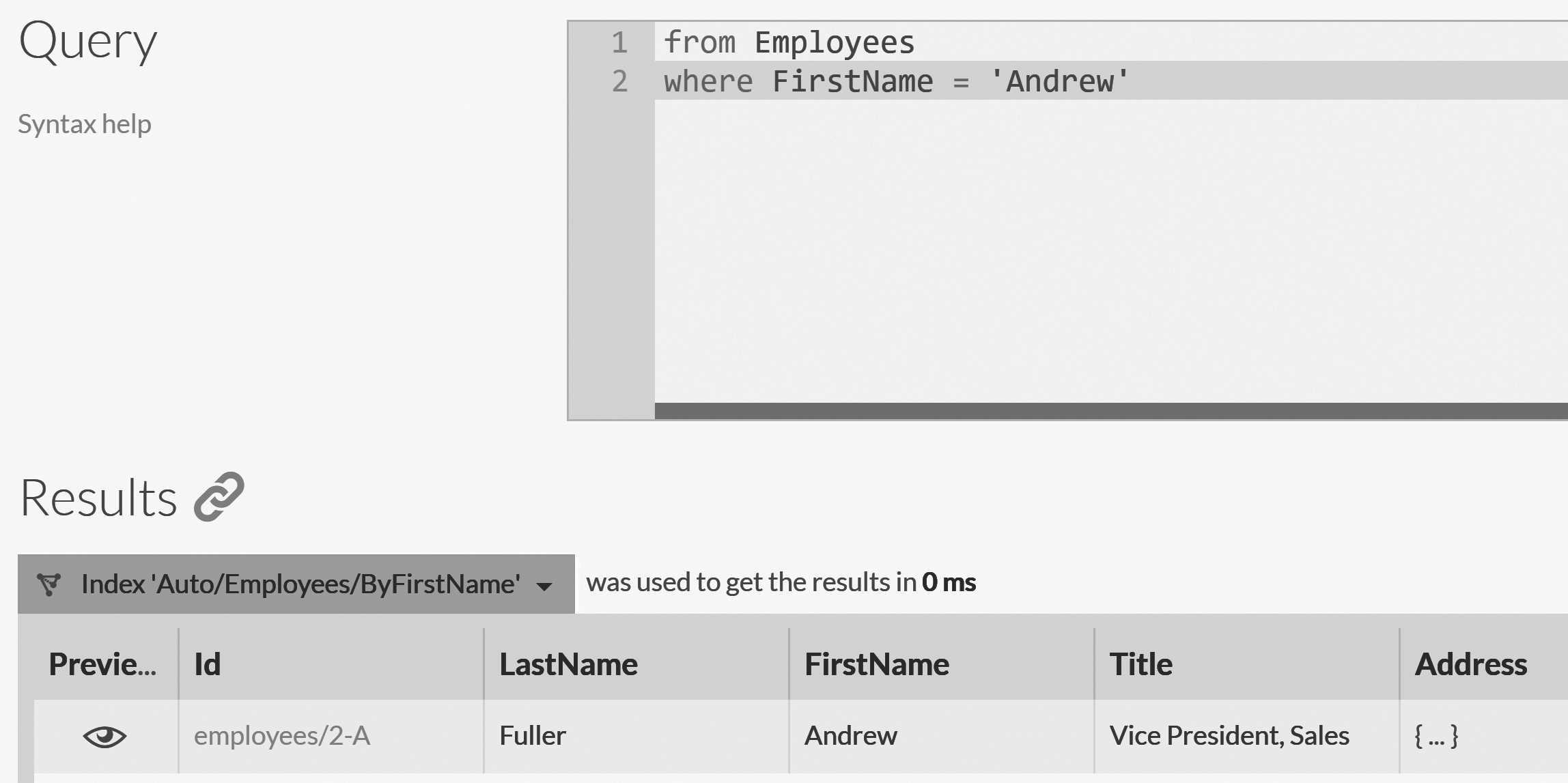
However, what happens when we start querying using the data itself? You can see the result in Figure 9.1. In particular, you'll note that RavenDB reports that this query used the Auto/Employees/ByFirstName index.

Switching over to the indexes listing will show you that, indeed, a new auto index was created to answer these kinds of queries. Let's test this further and query by last name now, using the following:

from Employees where LastName = 'Fuller'

You can see the index that was created as a result of running this query in Figure 9.2.

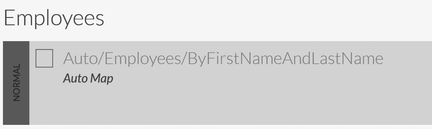
The query optimizer has detected that there's no index for this query, looked at the previous history of queries on the Employees collection and created an index that can satisfy all such queries in the future. If you were fast enough, you might have managed to catch the Auto/Employees/ByFirstName index disappearing as it was superseded by the new index.

Now that you've experienced the query optimizer firsthand, let's give it a bit of a workout, shall we? Let's see what kind of queries we can do with RavenDB.

The RavenDB Query Language

We decided to require that all queries must always use an index, and that decision has a few interesting results. It means that queries tend to be really fast because there's always an index backing the query and you don't need to go through full scans. Another aspect of this decision is that RavenDB only supports query operations that can be answered quickly using an index. For example, consider the following query:

from Employees where FirstName = 'Andrew'

This kind of query is easy to answer using an index that has indexed the FirstName field because we can find the Andrew entry and get all the documents that have this value. However, a query like the following is not permitted:

from Employees where years(now() - Birthday) > 18

This query would require RavenDB to perform computation during execution, forcing us to do a full scan of the results and evaluate each one in turn. That isn't a good idea if you want fast queries, and RavenDB simply does not allow them. You can rewrite the previous query to efficiently use the index by slightly modifying what you're searching for:

from Employees where Birthday < $eighteenYearsAgo

The $eighteenYearsAgo variable would be set for the proper time, and that would allow the database to find the results by merely seeking in the index and returning all the results smaller than the given date. That's cheap to do, and it's the proper way to run such queries. In general, you can usually do a straightforward translation between queries that require computations and queries that don't, as above. Sometimes you can't just modify the query. You need to tell RavenDB it needs to do some computation during the indexing process. We'll see how that's done in Chapter 10.

Queries can also use more then a single field, as you can see in Listing 9.2.

Listing 9.2 Querying over several fields at the same time

from Employees 
where (FirstName = 'Andrew' or LastName = 'Callahan') 
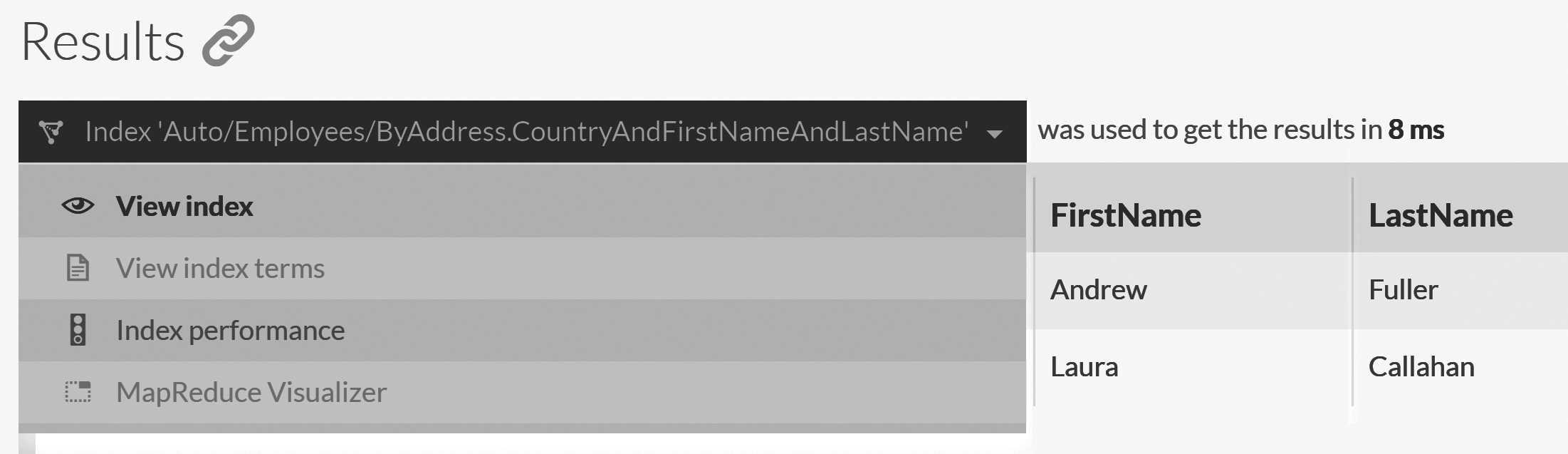
and Address.Country = 'USA'

Using the sample data set, this should give two results, as shown in Figure 9.3. In that figure, you can also see some of the options available to inspect the index behavior. Viewing the index definition will tell you what is indexed and how. And the indexing performance statistics will give you all the details about the costs of indexing, broken down by step and action. This is very important if you're trying to understand what is consuming system resources, but that will be covered in the next part of the book, discussing production deployments and how to monitor and manage RavenDB in production.

Far more important for us at this point is the View index terms page, which exposes the internal index structure. This is helpful when you need to understand how RavenDB is processing a query. If you click the View index terms link, you'll be taken to the index terms page, where you'll see the index fields. Clicking this will show you what was actually indexed, as illustrated in Figure 9.4.

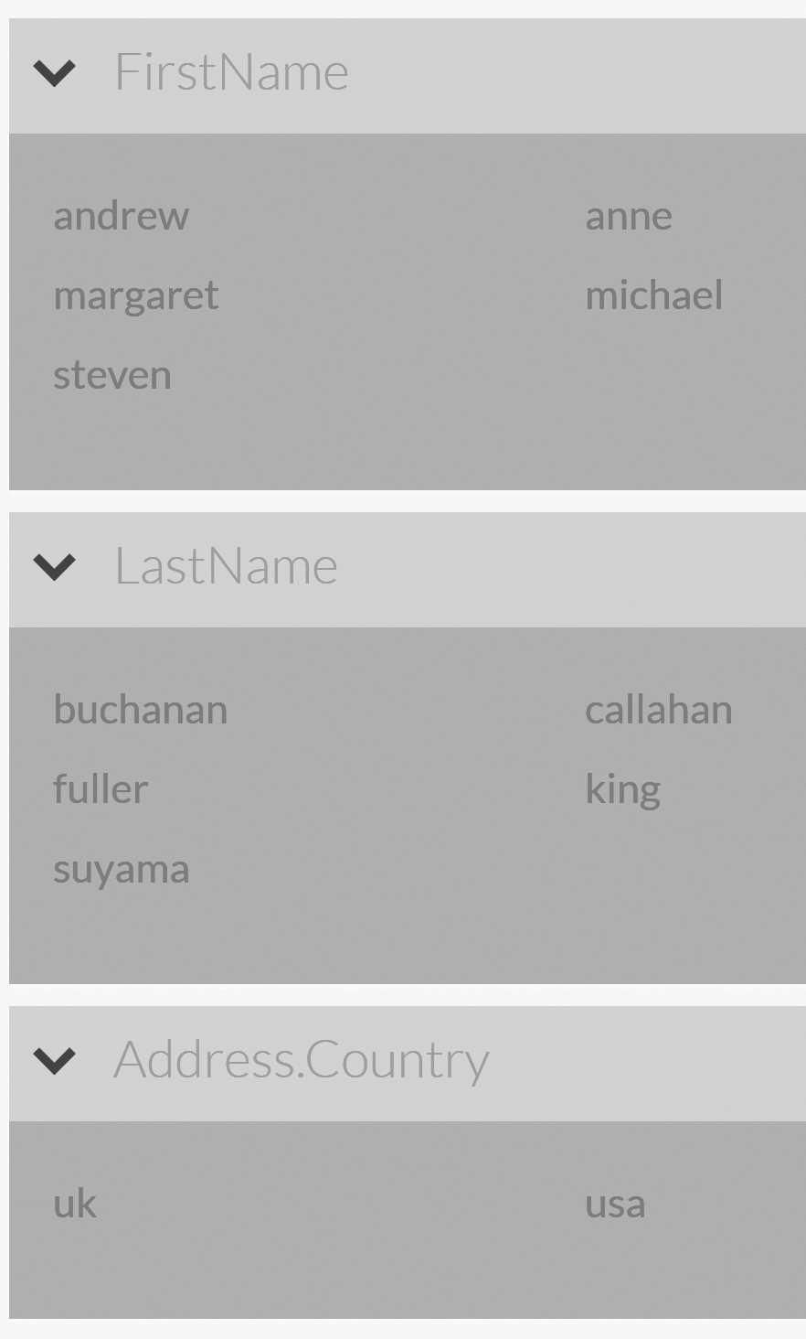
Why is this so important? Even though Figure 9.4 doesn't show all the values, it shows enough to explain how RavenDB will actually process the query. The first thing to understand is that RavenDB is going to treat each field in the query separately. The query is broken into three clauses, and you can see the result of each in Table 9.1.

Query	Results
FirstName = 'Andrew'	employees/2-A
LastName = 'Callahan'	employees/8-A
Address.Country = 'USA'	employees/1-A, employees/2-A, employees/3-A,
	employees/4-A, employees/8-A

Table: Query clauses and their individual results

The reason that RavenDB deals with each field separately is because it stores the indexed data for each field independently. This allows us a lot more freedom at query time, at the expense of having to do a bit more work.

RavenDB's indexes aren't single-purpose

If you're familiar with common indexing techniques in databases, you know there's a major importance to the order of the fields in the index. The simplest example I can think of is the phone book, which is basically an index to search for people by "LastName, FirstName."

If you have both a first and last name, then the phone book is easy to search. If you need to search just by last name, the phone book is still useful. If you only have a first name, however, the phone book is basically useless. You'll have to go through the entire thing to find any results.

In the same way, indexes that mash all fields together into a single key and then allow searching on the result are very efficient in answering that particular kind of query, but they can't really be used for anything else. With RavenDB, we index each field independently and merge the results at query time. That means that our indexes can be used in a more versatile manner, and they're able to answer a much wider range of queries at a small cost of additional work to merge them at query time.

To answer the query in Listing 9.2, RavenDB will find the matching documents for each of the clauses, as shown in Table 9.1. At that point, we can use set operations to find the final result of the query. We have an OR between the FirstName and LastName query, so the result of both clauses is the union of their results. In other words, the answer to FirstName = 'Andrew' or LastName = 'Callahan' is (employees/2-A, employees/8-A).

The next step in the query is to evaluate the and with the Address.Country = 'USA' clause. Because we have an and here, we'll use set intersection instead of a union (which we use for or). The result of that will be (employees/2-A,employees/8-A), which appear on both sides of the and. Similarly, and not uses set difference.

The end result is that a single index in RavenDB is able to be used by far more types of queries than a similar index in a relational database. This is at the cost of doing set operations on queries that have multiple clauses. Since set operations are quite cheap and have been carefully optimized, that's a pretty good tradeoff to make.

Operations in queries

As I mentioned, queries in RavenDB do not allow computation. We saw some simple queries earlier using equality and range queries at a glance. In this section, I want to talk about what kinds of queries you can make in RavenDB and dig a bit into how they're actually implemented.

The standard query operations you would expect are here, of course, as well as a few more, as shown in Table 9.2.

Operation	Operators / Methods
Equality	=, ==, !=, <>, IN, ALL IN
Range queries	>, <, >=, <=, BETWEEN
Text search	Exact, StartsWith, EndsWith, Search
Aggregation	Count, Sum, Avg
Spatial	spatial.Contains, spatial.Within, spatial.Intersects
Other	Exists, Lucene, Boost

Table: Operators and methods that can be used in queries

Equality comparisons

The first and most obvious operators are equality comparisons ('=' or '=='). As you can imagine, these are the easiest ones for us to find since we can just check the index for the value we compare against. It is important to note that we only allow the comparison of fields against values or parameters. This kind of query is fine: where FirstName = 'Andrew' as well as this: where FirstName = $name. However, this is not allowed: where FirstName = LastName.

These type of queries count as computation during a query and can't be expressed directly in RQL. Don't worry — you can still make such queries, but you need to use a static index to do that. This will be discussed in Chapter 10, which is dedicated just to this topic.

Inequality queries are more interesting. Remember that RavenDB uses set operations to compute query results. A query such as where FirstName != 'Andrew' is actually translated to: where exists(FirstName) and not FirstName = 'Andrew'. In other words, you're saying,"Find all the documents that have a FirstName field and exclude all the documents where that FirstName is set to 'Andrew'."

There's also IN, which can be used in queries such as where Address.City IN ('London', 'New York') — a shorter way to write where Address.City = 'London' or Address.City = 'New York'. However, IN also allows you to send an array argument and write the query simply as where Address.City IN ($cities), which is quite nice. ALL IN, on the other hand, is a much stranger beast. Quite simply, if we used ALL IN instead of IN, the query it would match is where Address.City = 'London' and Address.City = 'New York'. In other words, it'll use and instead of or. This is a strange and seemingly useless feature. How can a value be equal to multiple different values?

The answer is that a single value can't, but an array most certainly can. Consider the document shown in Figure 9.5, with an array of territories. We can use ALL IN in our query to find all the regions that have multiple territories in them, like so: from Regions where Territories[].Name ALL IN ('Wilton', 'Neward')

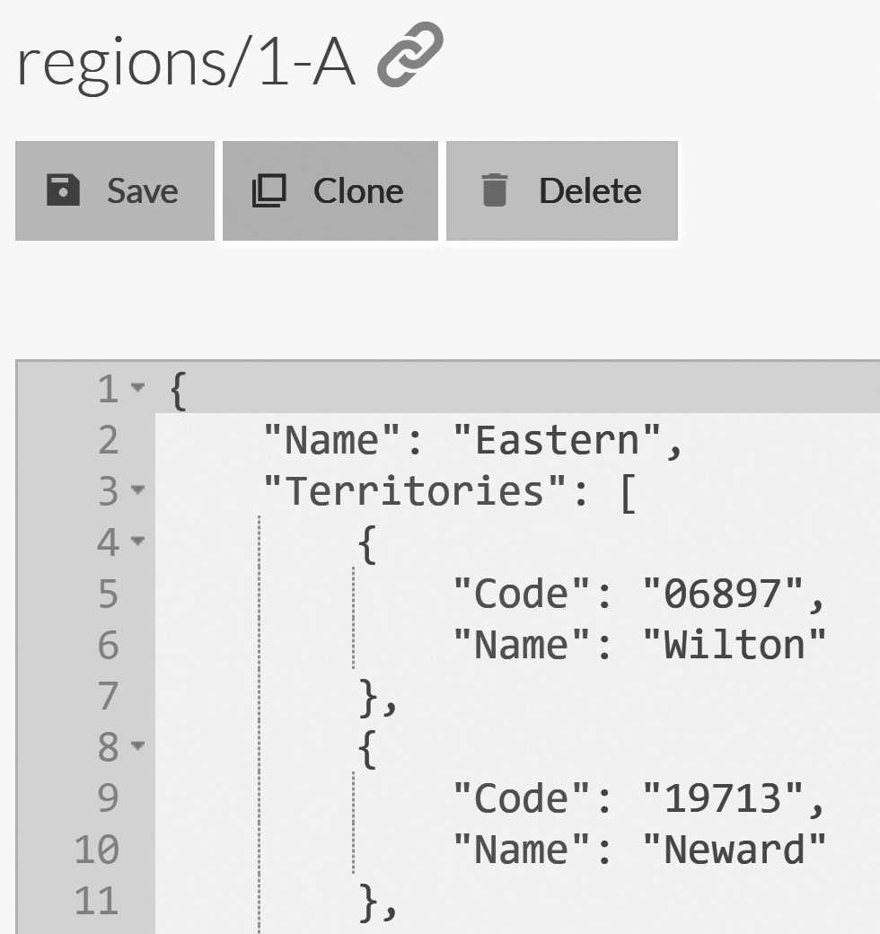
This query shows two new features. First, we have ALL IN, which shows how we can match multiple values against an array. A common usage of this feature is to filter documents by tags. The user can select what tags they're interested in, and you use ALL IN to find all the documents that match the requested tags.

The second new feature is the usage of the Territories[].Name path and, in particular, the use of [] in the path. Within RQL, the use of the [] suffix in a property indicates that this is an array and the rest of the expression is nested into the values of the array. This is useful both in the where clause and when doing projections using select, as we'll see later in this chapter.

Range queries

For range queries, things like > or <= are fairly self explanatory, with BETWEEN as a nicer mechanism for actually querying over a specific range. BETWEEN is inclusive on the low and high ends. In other words, consider the query in Listing 9.3.

Listing 9.3 Querying date ranges using BETWEEN

from Employees 
where HiredAt.Year BETWEEN 1992 AND 1994

The results of the query in Listing 9.3 will include employees hired in 1992, 1993 and 1994. We could have also written the same query with string matches, as shown in Listing 9.4.

Listing 9.4 Querying date ranges using BETWEEN with string prefixes

from Employees 
where HiredAt BETWEEN '1992' AND '1995'

The query in Listing 9.4 will also match all the employees hired in 1992, 1993 and 1994. But why? It's because of a minor trick we use here. The actual date format used by RavenDB is ISO 8601, so technically speaking, the query in Listing 9.4 is supposed to look like this: HiredAt BETWEEN '1992-01-01T00:00:00.0000000' AND '1995-01-01T00:00:00.0000000'. In practice, RavenDB considers such queries as string operations and allows us to do the BETWEEN operation using just the prefix.

This is because of the way RavenDB processes range queries. For non-numeric values, range queries use lexical comparisons, which means that just specifying the prefix is enough for us to get the required results. That's why RavenDB uses ISO 8601 dates. They sort lexically, which makes things easier all around at querying time.

For numeric values, we use the actual number, of course. That too, however, has some details you should be familiar with. When RavenDB indexes a numeric value, it will actually index that value multiple times: once as a string, which allows it to take part in lexical comparisons, and once as a numeric value. Actually, it's even more complex than that. The problem is that when we deal with computers, defining a number is actually a bit complex.

Range queries on mixed numeric types

If you use the wrong numeric type when querying, you'll encounter an interesting pitfall. For example, consider the products/68-A document in the sample dataset. Its PricePerUnit is set to 12.5; yet if we query for from Products where PricePerUnit > 12 and PricePerUnit < 13, RavenDB finds no results.

The problem is that we're using an int64 with a range query, but PricePerUnit is actually a double. In this case, RavenDB indexed the PricePerUnit field as both double and int64. However, when indexing the 12.5 value as int64, the value was naturally truncated to 12, and the query clearly states that we want to search for values greater than 12, so RavenDB skips it.

A small change to the query, from Products where PricePerUnit > 12.0 and PricePerUnit < 13.0 will fix this issue.

RavenDB supports two numeric types: 64-bit integers and IEEE 754 double-precision floating-points. When RavenDB indexes a numeric field, it actually indexes it three times: once as a string, once as a double and once as an int64. And it allows you to query over all of them without really caring what you use to find your results.

Full text searching

So far, we've looked at querying the data exactly as it is. But what would happen if we ran the following query?

from Employees where FirstName = 'ANDREW'

Unlike the previous times we ran this query, now the FirstName is using a different case than the value of the field in the document. But we'd still get the expected result. Queries that require you to match case have their place, but they tend to be quite frustrating for users. So RavenDB defaults to using case-insensitive matching in queries.

On the other hand, you could have written the query as shown in Listing 9.5 and found only the results that match the value and the casing used.

Listing 9.5 Case sensitive queries using the exact() method

from Employees 
where exact(FirstName = 'Andrew')

Within the scope of the exact, you'll find that all comparisons are using case-sensitive matches. This can be useful if you're comparing BASE64 encoded strings that are case sensitive, but it's rarely useful otherwise.

By default, queries in RavenDB are case insensitive, which helps a lot. But what happens when we need more than a match? Well, we can use StartsWith and EndsWith to deal with such queries. Consider the following query:

from Employees where StartsWith(FirstName, 'An')

This will find all the employees whose names start with 'An'. The same can be done with where EndsWith(LastName, 'er') for the other side.

Note that queries using StartsWith can use the index efficiently to perform prefix search, but EndsWith is something that will cause RavenDB to perform a full index scan. As such, EndsWith isn't recommended for general use. If you really need this feature, you can use a static index to index the reverse of the field you're searching on and use StartsWith, which will be much faster.

Of more interest to us is the ability to perform full text searches on the data. Full text search allows us to search for a particular term (or terms) in a set of documents and find results without having an exact match. For example, examine Figure 9.6, where we're searching for a company that has the word 'stop' in its name.

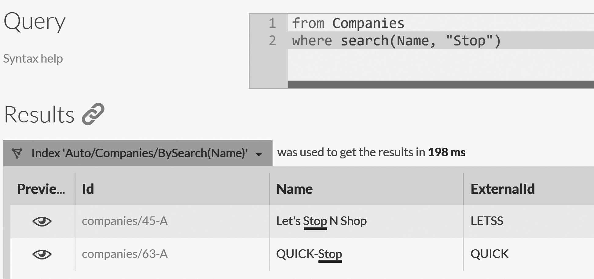
The result of this query is that we're able to find two results. What makes this interesting is that, unlike the EndsWith case, RavenDB didn't have to go through the entire result set. Let's go into the terms for the Auto/Companies/BySearch(Name) index and see how this works.

We have two fields indexed here. The first is Name, and if you click on that, you'll see 91 results — one for each of the companies we have in the sample dataset. The other one is named search(Name) and is far more interesting. Clicking on it shows 223 results, and the terms that are indexed are not the names of the companies. Figure 9.7 shows a comparison of the two fields.

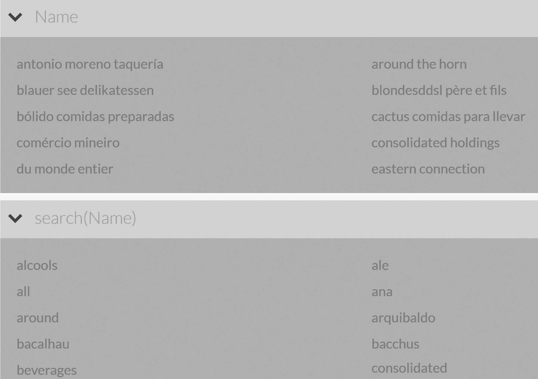
When we do a simple equality query, such as where Name = 'Consolidated Holdings', it's easy to understand how the database will execute this query. The Name field's terms are sorted, and we can do a binary search on the data to find all the documents whose name is equal to "Consolidated Holdings". But what happens when we query using search(Name)?

The answer is in the way RavenDB indexes the data. Instead of indexing the Name field as a single value, RavenDB will break it into separate tokens, which you can see in Figure 9.7. This means that we can search for individual words inside the terms. We search not the full field but rather the indexed tokens, and from there, we get to the matching documents.

Full text search is a world unto itself

I'm intentionally not going too deep into full text search and how it works. If you're interested in learning more about full text search, and I personally find the topic fascinating, I recommend reading Lucene in Action and Managing Gigabytes. They're both good books that can give you insight into how full text search works. Lucene in Action will give you a practical overview. Managing Gigabytes is older (it was written about twenty years ago), but it's more digestible for handling the theory of full text search. These books aren't required reading for understanding how to use RavenDB, though.

Most of the work was already done during the indexing process, so queries tend to be very fast. Full text search in RavenDB also allows us to do some fascinating things. For example, consider the following query:

from Companies where search(Address, "London Sweden")

The Address property on the Companies documents isn't a simple string; it's actually a nested object. But RavenDB has no problems indexing the entire object. The results of this query include companies that reside in the city of London or in the country of Sweden. This powerful option allows you to search across complex objects easily.

It's worth noting the order in which the results have returned from the query. In order to better see that, we'll use a select clause (we'll talk about that more later in this chapter) to fetch just the information we're interested in. See Listing 9.6 for the full query.

Listing 9.6 Full text search and projection on the relevant fields

from Companies 
where search(Address, "London Sweden")
select Address.City, Address.Country

The results of the query in Listing 9.6 are really interesting. First, we have six companies that are located in London. Then we have two that are based in Sweden. Here's the interesting part: this isn't accidental. RavenDB ranks the results based on their quality. A match on London would rank higher than a match on Sweden since London was the first term in the query. (Switch them around and see the change in results). This means the more relevant results are nearer to the top and more likely to be seen by a user.

Lucene

RavenDB uses the Apache Lucene library for indexing, which means that there's quite a bit of power packed behind these indexes. Lucene is a full text search library that can support complex queries and is considered to be the de facto leader in the area of search and indexing.

Unfortunately, Lucene is also temperamental. It's tricky to get quite right, and it's not known for its ease of use or robustness in production systems. Even still, this library is amazing, and whenever you run into search anywhere, it's a safe bet that Lucene is the core engine behind it. For that reason, it's common to consume Lucene using a solution that wraps and handles all of the details of managing it (such as Apache Solr or ElasticSearch).

In the case of RavenDB, a major factor in our Lucene usage is that we're able to have our storage engine (Voron) provide transactional guarantees, which means our Lucene indexes are also properly ACID and safe from corruption without us needing to sacrifice expected performance. In general, all the operational aspects of running Lucene indexes are handled for you, and they shouldn't really concern you. We'll discuss Lucene in more depth in Chapter 10. But for now, I want to focus on the querying capabilities that Lucene provides.

If you're familiar with Lucene, you might have noticed that RQL is nothing like the Lucene query syntax. This is intentional. Lucene queries only find matches, while all else, like sorting of projections, is handled via code. This makes it a great tool for finding information but a poor tool for actual queries. That said, you can use an RQL query and the Lucene method as an escape hatch to send queries directly to Lucene.

The following query uses the Lucene method to query with wildcards, which isn't supported by RavenDB.

from Companies where Lucene (ExternalId, "AL?K?") 

There are some scenarios where this is required, particularly if you're upgrading an application from older versions of RavenDB, which exposed the Lucene syntax directly to users. But in general, RQL should be sufficient and is the recommended approach. Typically, you'd only use Lucene on static indexes where you have control over what fields are indexed.

Built-in methods in RQL are case insensitive

Built-in methods (such as the ones listed in Table 9.2) are case insensitive, and you can call where startsWith(Name, 'An') or where StartsWith(Name, 'AN') without issue. Note that field names are case sensitive, though.

Most of what you can do with Lucene is available natively in RQL. For example, we can use the Boost() method to change the way queries are evaluated. Consider the query in Listing 9.7, which expresses a fairly complex conditional and ranking requirement using Boost()

Listing 9.7 Using boost to modify query results ranking

from Companies
where Boost(Address.City = 'London', 3) or
      Boost(Address.City = 'Paris', 2) or
      Address.Country IN ('Germany', 'Sweden')

The query in Listing 9.7 will select companies based in London, Paris or anywhere in Germany or Sweden. The effect of Boost() on the results is that a document matching on London would be given a boost factor in the ranking. This means that the query in Listing 9.6 will first get results for London, then Paris and then Germany and Sweden.

This may seem silly, but there are many search scenarios where this can be a crucial feature. Consider searching on messages. A match on the Subject field is more important than matches on the Body field, but we want to get results from both.

An interesting issue with boosting is that it isn't quite as obvious as you may think. Consider the query in Listing 9.7. If we change the last clause to be Address.Country IN ('Germany', 'France'), we'll start getting Parisian companies first, even though the boost on London-based companies is higher. The reason for that is because the Parisian companies will have two matches to their names (both Paris and France) while the London companies will only have one. The results from Paris will be considered higher quality and be ranked first.

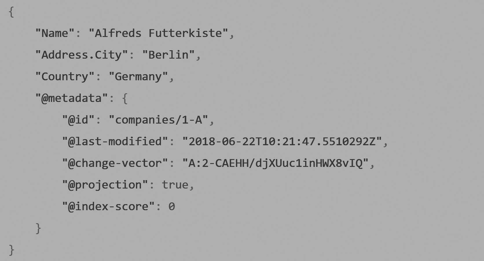
Exposing the raw score

The query result also includes the @index-score metadata property that exposes the scoring of each result. You can inspect this to figure out why the final sort order of a query is the way it is.

We could adjust that by increasing the boost factor for the London-based companies, but in more complex scenarios, it can be hard to figure out the appropriate ratios. In practice, when using such techniques, we aren't usually too concerned with absolute ordering. The expected consumer of these sorts of queries is the end user, who can scan and interpret the information as long as the ranking more or less makes sense.

Projecting results

We've looked into how to filter the results of a query, but so far, we've always pulled the full document back from the server. In many cases, this is what you want to do. In Chapter 3, we spent a lot of time discussing how you should think about documents. One element of the trifecta of document modeling (cohesive, coherent and isolated) is the notion that a document is cohesive. From a modeling perspective, it doesn't usually make sense to just grab some pieces of data from a document without having it all there.

At least, it doesn't make sense until you realize that you often need to display the data to the user, picking and choosing what will be shown. For example, an order without its order lines may not be very meaningful in a business sense to the user. But knowing that an order was made on December 17th is probably enough information to recall they required expedited shipping on their last-minute holiday shopping to get it in time.

In this section, we're going to take documents apart and then mash them together. In almost all cases, projection queries are used for either subscriptions or for feeding the data into some sort of a user interface. If you need to actually work with the data, it's generally better to get the full document from the server and use that. It's also important to remember that on the client side, projections are not tracked by the session, and modifications to a projection will not modify the document when SaveChanges is called.

The simplest query projection can be seen in Listing 9.8.

Listing 9.8 Projecting only some parts of the document

from Companies
select Name, Address.City, Address.Country as Country

The query in Listing 9.8 will produce the results with three fields: Name, Address.City and Country. A single simple projection of fields and the use of aliases from this query is demonstrated in Figure 9.8. You can see that we didn't specify an alias for the Address.City field and that the full name was used in the resulting projection. On the other hand, the use of aliases, as we can see in the case of Country, allows us to control the name of the field that would be returned.

In the case of the query in Listing 9.8, we're only projecting simple fields, but RQL is capable of much more. Listing 9.9 has a more complex projection example, projecting both objects and arrays.

Listing 9.9 Projecting arrays and objects using RQL

from Orders
select ShipTo, Lines[].ProductName as Products

A single projection from the results of the query in Listing 9.9 is shown in Figure 9.9. This query is a lot more fun. You can see that there's no need to flatten out the query and that we can send complex results back. The projection of Lines[].ProductName is more interesting. Not only are we projecting an array, but we're actually projecting a single value from the array back to the user. I don't think that I need to expand on how powerful such a feature can be.

The select clause listing is an easy, familiar way to get a specific piece of data out. But it only lets us select what we're getting back and rename it using aliases. RavenDB is a JSON database, and as smart as the select is, it's best for dealing with mostly flat data. That's why we have the ability to project object literals.

Projecting with object literals

SQL was meant to handle tabular data. As such, it's great in expressing tabular data but not so great when we need to work with anything but the most trivial of documents. With RQL, you aren't limited to simply selecting the flat list of properties from the document. You can also project a complex result with the object literal syntax. Let's look at a simple example of using object literals to query in Listing 9.10.

Listing 9.10 RQL projection using object literal syntax

from Orders as o
select {
    Country: o.ShipTo.Country,
    FirstProduct: o.Lines[0].ProductName,
    LastProduct:  o.Lines[o.Lines.length - 1].ProductName,
}

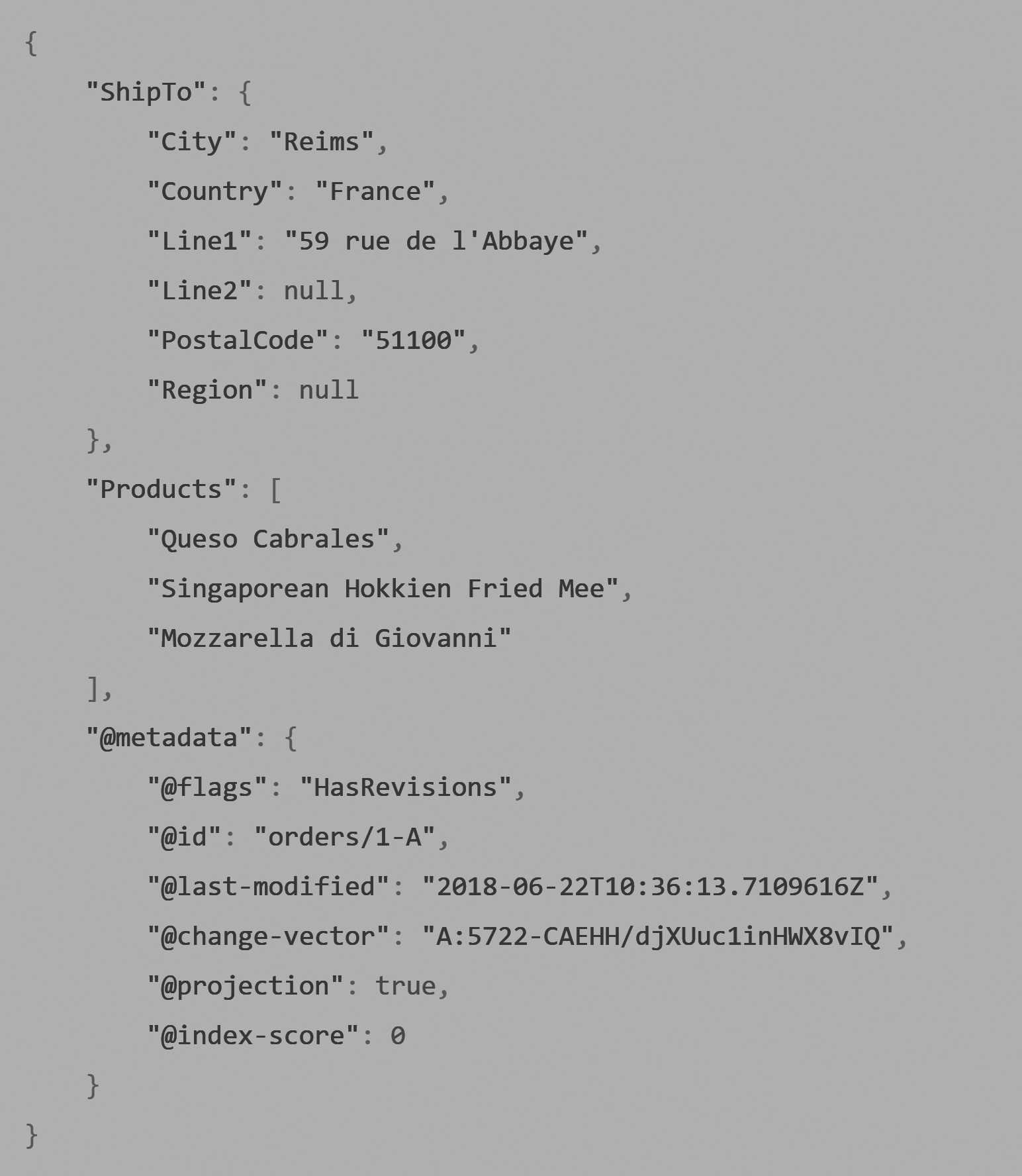
The result of the query in Listing 9.10 for document orders/1-A is shown in Listing 9.10. As you can see, we're able to project the data out not only using property paths but also using complex expression, pulling the first and last products from the order.

Alias is required with the object literal syntax

The query in Listing 9.10 is using from Orders as o, defining the alias o for the Orders collection. This is required when using the object literal syntax since we need to know the root object the expression starts from.

Listing 9.11 Result of projection from Listing 9.10

{
    "Country": "France",
    "FirstProduct": "Queso Cabrales",
    "LastProduct": "Mozzarella di Giovanni",
    "@metadata": {
        "@id": "orders/1-A",
    }
}

The key to the object literal syntax is that this isn't a JSON expression; it's a JavaScript object literal, and any valid JavaScript expression is going to work. For example, let's take a look at Listing 9.12, which shows a slightly more complex example.

Listing 9.12 Projections of JavaScript metohd calls

from Orders as o
select {
    Year: new Date(o.ShippedAt).getFullYear(),
    Id: id(o)
}

Because JSON doesn't have a way to express dates natively, we can use the new Date().getFullYear() to handle date parsing and extracting of the year portion of the date. You can see the projection of the document identifier as well. In addition to the usual JavaScript methods, you also have access to functions defined by RavenDB itself, such as id. A full list of the functions available for your use can be found in RavenDB's online documentation.

We'll look at one final example of the kind of projections you can make with the object literal syntax, mostly because I think it's a beautiful example of what you can do. Listing 9.13 shows a query that will get the two most expensive products and the total value of the order.

Listing 9.13 Making non trival calculations in projections

from Orders as o
select {
    TopProducts: o.Lines
        .sort((a, b) => 
            (b.PricePerUnit * b.Quantity) - 
                (a.PricePerUnit * a.Quantity))
        .map(x => x.ProductName)
        .slice(0,2),
    Total: o.Lines.reduce(
        (acc, l) => acc += l.PricePerUnit * l.Quantity, 0)
}

There's a lot going on in this small bit of code, so let's break it into its individual pieces. First, we use the object literal syntax and define two properties that we'll return. For TopProducts, we sort the lines by the PricePerUnit * Quantity in descending order, grabbing just the names, and then take the first two items. For Total, we simply use the JavaScript reduce method to calculate the total price on the order during the query. If you're familiar with JavaScript, this is nothing special, but it expresses a lot of the power available to you when you project using the object literal syntax.

The object literal syntax is quite flexible, but it has a few limits. In particular, take a look at Listing 9.13 and how we compute the cost of a particular product by using the following formula: l.PricePerUnit * l.Quantity. However, I forgot to also include the discount that may be applied here. The formula for the discount is simple. The new way to compute the price of a product is simply l.PricePerUnit * l.Quantity * (1 -l.Discount). That's easy enough, but it repeats three times in Listing 9.13, making it a perfect example of a violation of the "don't repeat yourself" principle. If we were writing code using any standard programming language, we would wrap this in a function call to make it easier to understand and so that we would only need to change it in a single location. Luckily, RQL also has such a provision, and it allows you to define functions.

Listing 9.14 shows how we can use the function declaration to properly compute the product price while avoiding repetition.

Listing 9.14 Using functions to consolidate logic

declare function lineItemPrice(l) {
    return l.PricePerUnit * l.Quantity * (1 - l.Discount);
}
from Orders as o
select {
    TopProducts: o.Lines
        .sort((a, b) => lineItemPrice(b) - lineItemPrice(a) )
        .map(x => x.ProductName)
        .slice(0,2),
    Total: o.Lines.reduce((acc, l) => acc + lineItemPrice(l), 0)
}

In Listing 9.14, we first declared the function lineItemPrice. This took the line item and computed the total amount you would pay for it. Once this was declared, you could then use the function inside the object literal.

Declaring functions in queries

You can declare zero or more functions as part of the query, and they will be visible both to each other and to the object literal expression. Such functions can do anything you want, subject to the usual limits of projections. (You can't take too long to run since it will time out the query).

Inside the function, all the usual JavaScript rules apply, with the exception that we'll ignore missing properties by default. In other words, you can write code such as l.Who.Is.There, and instead of throwing a TypeError, the entire expression will be evaluated to undefined.

Declared functions can only be used from inside the object literal expression and are not available for the simple select expression syntax.

I'm sure you can imagine the kind of queries that declaring functions make possible. You can tailor the results of the query specifically to what you want, and you can do all that work on the server side without having to send a lot of data over the wire.

Projections are applied as the last stage in the query

It's important to understand that projections—either simple via select Name, Address.City, Address.Country as Country or more complex using the object literal syntax— are applied as the last stage in the query pipeline. In other words, they're applied after the query has been processed, filtered, sorted and paged. This means that the projection doesn't apply to all the documents in the database, only to the results that are actually returned.

This reduces the load on the server significantly since we can avoid doing work only to throw it out immediately after. And it also means that we can't do any filtering work as part of the projection. You can filter what will be returned but not which documents will be returned. That has already been determined earlier in the query pipeline.

Another consideration to take into account is the cost of running the projection. It's possible to make the projection query expensive to run, especially with object literal syntax and with method declarations that we'll soon explore. RavenDB has limits to the amount of time it will spend evaluating the projection, and exceeding these (quite generous) limits will fail the query.

I want to emphasize that you shouldn't be reluctant to use projections or the object literal syntax in particular. This can significantly reduce the amount of data that's sent over the network, and it's usually preferred when you need to return a list of documents showing only partial data for display purposes.

In fact, there's one more way to project data from queries: using a function directly. This method is usually employed when you want to return objects with a different shape in the query. Before we see how this can be done, a word of caution; it's usually hard to deal with heterogeneous query results, with each object being a potentially different shape. There are some cases where this is exactly what you want, but it usually complicates the client code and shouldn't be overused.

Listing 9.15 shows how we can project a method directly to the client, doing what's probably the world's most ridiculous localization effort.

Listing 9.15 Returning differently shaped results based on the document data

declare function localizedResults(c) {
    switch(c.Address.Country)
    {
        case "France":
            return { Nom: c.Name };
        case "Brazil": 
            return { Nome: c.Name };
        default:
            return { Name: c.Name };
    }
}
from Companies as c
where id() in ('companies/15-A', 'companies/14-A', 'companies/9-A')
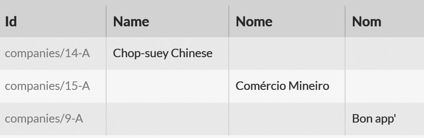
select localizedResults(c)

The result of this query can be seen in Figure 9.10, where you can see that different documents have different shapes. I had a lot of fun writing the query in Listing 9.15, but I wouldn't want to have to deal with it in my code. It would probably be too confusing.

To summarize projections, we have the following options available to us when we query RavenDB.

• Getting the whole document back. This can be done by omitting the select clause entirely or using select o or select *, with o being the root alias of the query.
• Projecting values from the document using simple select expressions, such as select Name, Address.City, Address.Country as Country. This allows us to control what's sent back and lets us rename fields. We can also project nested values and dig into arrays and objects, but this is intentionally made simple to ensure that we can process it quickly and efficiently.
• Projecting values from the document using object literal expression gives you far more power and flexibility. You can utilize JavaScript expressions to get the results just the way you want them. This includes doing computation on the returned result set and even declaring functions and doing more work inside the function to avoid repetition and to make it easy to build complex queries.
• Projection values as the result of a single method call in the select, such as select localizedResults(c). In this case, the shape and structure that will be returned is completely up to you. You can even return null or undefined from the method call, and that will be sent to the client (where you'll need to be careful about handling it, of course).

Of the four options we have, you need to remember that only the first option will give you the full document back. In all other cases, you'll be returning a projection. This is important from the client side because the client API won't be tracking a projection, and changes to the projection will not be saved back to the server when you call SaveChanges.

Querying by ID

If you look at Listing 9.15, you'll see an interesting type of query. There, we're querying by document ID and specifying a projection. This may seem like a strange thing to do. Surely it'd be better to just get the documents directly if we know what their IDs are, no?

Querying by ID is handled differently. If the query optimizer can see that your query is using an ID, then instead of going through an index, it'll fetch the relevant documents directly using their IDs and pass them to the rest of the query for processing. This applies when you're querying by ID and don't have additional filters, sorting or the like that would require the use of an index.

This allows us to define projections on a single document (or a group of them) and use all the power of RQL projections to get back the results we want. For large documents, this can be significant savings in the amount of data that goes over the network. And that's without the server having to make any additional effort since this is an exception to the rule that queries without an index to cover them will have an index created for them. In this case, the query optimizer can use the internal storage indexes and avoid creating another one.

We looked into all the different ways we can project results from a document as part of a query, but there's still more we can do. We can use RQL to work with multiple documents. That's the topic of the next section.

Loading and including related documents

In general, queries in RavenDB apply only to a single document. That is, you can ask questions about a single document and not about other documents.

Querying on relations

The previous statement isn't quite true. You can actually query on related documents and even across heterogeneous document collections using RavenDB, but only when you're the one who's defining the index. We'll discuss static indexes in the next chapter, so I'll hold discussion of that until then.

In other words, you can query on every aspect of a document quite easily, but it's not trivial to query on related data. If you're used to SQL, then the simple answer is that RavenDB doesn't allow joins. Recall the three tenets of document design: coherent, cohesive and independent. With proper modeling, you shouldn't usually want to join. But RavenDB has ways to enable that scenario, and they're discussed in the next chapter.

That said, it can be very useful to grab some data from related documents during the query. Consider a query to show the list of recent orders. We can query it using from Orders where Company = 'companies/1-A', and the result is shown in Figure 9.11.

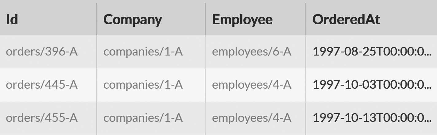
As you can see in Figure 9.11, the output is the document. That document includes useful fields such as Company and Employee. This is great, but if we intend to show it to a user, showing employees/6-A is not considered a friendly act. We can ask RavenDB to include the related documents as well, as you can see in Listing 9.16.

Listing 9.16 Including related documents in RQL

from Orders 
where Company = 'companies/1-A'
include Company, Employee

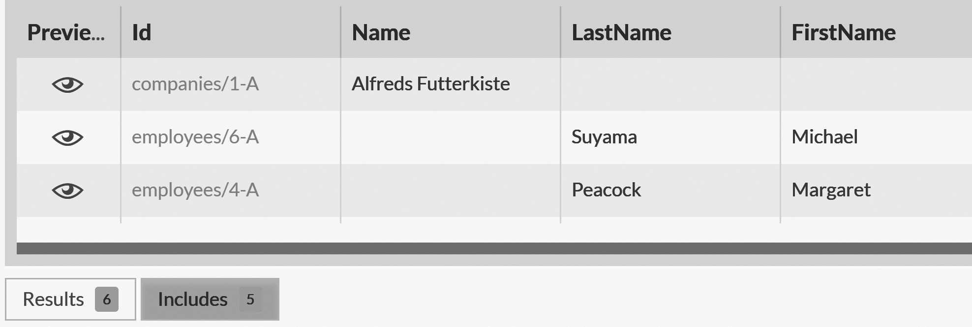
Figure 9.12 shows the output of this in the Studio, and you can see that we've gotten the company and the employees back from the query. We've already talked about the include feature in Chapter 4 at length. It allows us to ask RavenDB to send us related documents as well as the query results themselves, saving us the network roundtrip to fetch the additional information.

Including related documents is very useful, but if we just intend to show the information to the user, sending the full documents back can be a waste. We can do better by using load. In Listing 9.17, you can see a small example of pulling data from multiple documents and returning that to the user.

Listing 9.17 Using load to fetch data from related documents

from Orders as o
where Company = 'companies/1-A'
load o.Company as c, o.Employee as e
select {
    CompanyName: c.Name,
    EmployeeName: e.FirstName + " " + e.LastName,
    ShippedAt: o.ShippedAt
}

It's important to remember that the load clause is not a join; it's applied after the query has already run and before we send the interim results to the projection for the final result. Thus, it can't be used to filter the results of the query by loading related documents and filtering on their properties. It also means that load doesn't impact the cost of the query, and the database will only need to handle a single page of results to send back to the client.

You can also use the load() method inside declared functions or inside the object literal. We could have skipped the load o.Company as c and used CompanyName: load(o.Company).Name instead and gotten the same results. Load is also supported for collections, as you can see in Listing 9.18.

Listing 9.18 Loading data using arrays

from Orders as o
where Company = 'companies/1-A'
load o.Employee as e, o.Lines[].Product as products[]
select { 
    CompanyName: load(o.Company).Name,
    EmployeeName: e.FirstName + " " + e.LastName,
    ShippedAt: o.ShippedAt,
    Products: products
}

In Listing 9.18 we pull all the related products from the lines. Note that we indicate to RavenDB that the result is an array by using products[], but we use products in the object literal (since it's an array instance value there). The same would be the case for simple select. We don't need to specify the [] postfix for RavenDB to know that this is an array.

Loading documents in such a manner allows you to bring together a complete picture for the user. This is typically done as a way to feed the results directly from RavenDB to the UI, with minimal involvement of middleware between the UI and the results of the query. For includes, you're actually getting the real documents back. Modifications on them will be sent to the server when you call SaveChanges. But when you're using load, you'll typically get a projection back, which isn't tracked.

With load, you typically have fewer bytes going over the network, but sometimes it's easier to do certain things in your own code. Even though load and object literals allow you to shape your results in some pretty nifty ways, don't try to push too much into the database layer, especially if this is business logic. That road rarely leads to maintainable software systems.

Sorting query results

All the queries we've made so far have neglected to specify the sort order. As such, the order in which results are returned isn't well defined. It'll usually be whatever RavenDB thinks is the most suitable match for the query. That works if you're using queries that match over complex conditionals, but it's usually a poor user experience if you query for the orders a user made in the past six months.

RQL supports the order by clause, which allows you to dictate how results are sorted. Take a look at Listing 9.19 for an example.

Listing 9.19 Sorting by multiple fields in RQL

from Employees 
where Address.Country = 'USA'
order by FirstName asc, LastName asc

The query in Listing 9.19 reads like a typical SQL one, and that's by design. However, you need to be aware of a very important distinction. Consider the query in Listing 9.20.

Listing 9.20 Sorting by multiple fields in RQL with different orders

from Employees 
where Address.Country = 'USA'
order by LastName asc, FirstName asc

The query in Listing 9.20 is very nearly the same exact query as the one in Listing 9.19. However, the sort order is different. Why does this matter? It matters because, in both cases, we used the same index: "Auto/Employees/ByAddress.CountryAndFirstNameAndLastName," in this case. This is one of those cases where you needed to have experienced the pain to understand why this is such an important detail.

Typically, databases will use an indexing format that allows the database to quickly answer specific order by clauses. Similar to the phone book we discussed earlier in the chapter, they can only be used for the purpose for which they were created. It's possible to use the phone book index to answer the query in Listing 9.20, but it isn't in Listing 9.19. RavenDB, however, doesn't use such single purpose indexes. It indexes each field independently. That means it's able to answer both queries (and any combination thereof) using a single index.

The more flexible index and sorting behavior makes little difference if the size of the data is small. But as the size of the data increases, this means that you can still offer flexible sorting to the users, while other databases will typically be forced to do full table scans.

Another important factor of sorting in RavenDB is that it's applied after the filters. In fact, the RQL syntax has been designed so each step in the query pipeline corresponds to its place in the query as you type it. You can see that, in the queries in Listing 9.19 and 9.20, the order by comes after the where clause. That's because we first filter the result, and then we sort them.

This is more flexible, but it has a downside. If you're querying over a large dataset without a filter and you apply sorting, then RavenDB needs to sort all of the results and give you back just the first few records. This is usually only a problem if your query has hundreds of thousands of results to sort through. In such cases, it's usually advisable to filter the query to reduce the number of results that RavenDB needs to sort.

You aren't limited to sorting by the fields on the document. You also have the following sorting options:

• order by score() — order the results by how closely they match the where clause (useful if you are using full text search or using OR in the where clause).
• order by random() — random order, useful for selecting a random result from the query.
• order by spatial.distance() — useful for spatial queries which will be discussed later in this chapter.
• order by count() / order by sum() — allows ordering the results of queries using group by, discussed later in this chapter.

The sort order can also be impacted by how you want RavenDB to sort the fields. For example, consider the following query: from Products order by PricePerUnit desc. If you run it, you'll get some peculiar results, as shown in Figure 9.13.

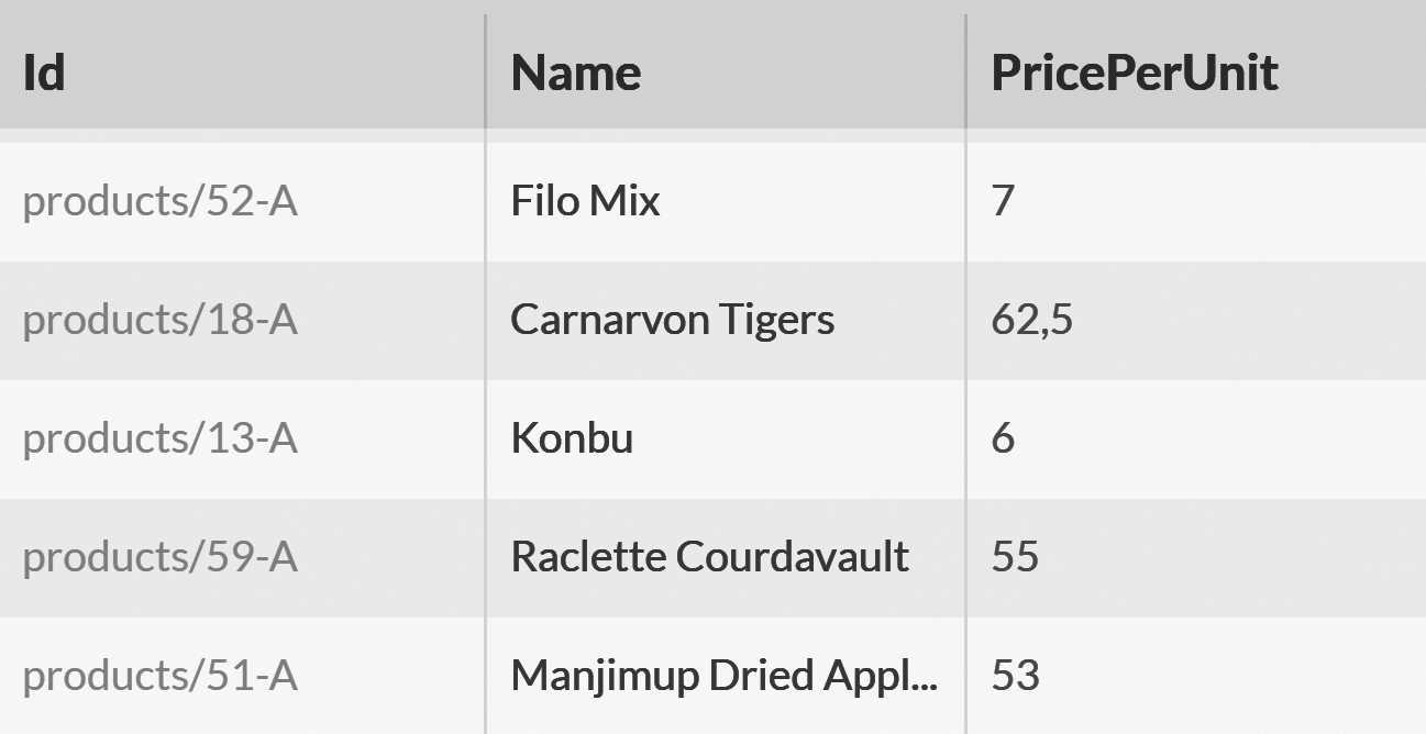
The issue is that RavenDB doesn’t know the type of the PricePerUnit field, and therefore it defaults to lexical ordering, which means that 7 will show before 62.5. In order to get the actual descending results from our order by clause, we need to let RavenDB know what kind of sorting we want to do. An example of how to do just that can be seen in Listing 9.21.

Listing 9.21 Sorting by numeric data in RQL

from Products
order by PricePerUnit as double desc

The as double in Listing 9.21 instructs RavenDB to sort the results as doubles. You can also use as long to specify that the data should be sorted as natural integers, truncating any fractional values. The way as long and as double work is they direct RavenDB to use a dedicated field with the numeric values in the index instead of using the string value for sorting. There's also the ability to sort using as alphanumeric, which will do exactly what you expect and apply alphanumeric sorting to the query.

Deep paging is discouraged

Sorting and paging usually go together. Paging is actually specified outside of RQL, so we won't be seeing it in this chapter. However, paging in RavenDB is pretty simple, in general. You specify the number of results you want and the number of results you want to skip. The first option, the number of results you want to get back, is obvious and easy for RavenDB to deal with. The second, not so much.

For example, if you want to get the first page, you specify start as 0 and pageSize as 10. If you want the second page, you specify that start is 10, and so on. This works well as long as the depth of your paging isn't too excessive. What do I mean by that?

If you expect to be issuing queries in which the start is very high (thousands or higher), you need to be aware that paging will happen during the sorting portion of processing the query. We'll get all the matching results for the query, sort them, and then select the relevant matches based on the page required.

However, the more deeply you page, the more work you force RavenDB to do. If you need to page deeply into a result set, it's typically much better to do the paging in the where clause. For example, if we were looking at recent orders for a customer and we expected customers to want to look at very old orders, we'd be better off specifying that the pages we show are actually dates. So the query will become where OrderedAt < $cutoffPoint. This will significantly reduce the amount of work required from RavenDB.

There isn't much more to say about sorting In RavenDB. It works pretty much as you would expect it to.

Spatial queries

Spatial searches allow you to search using geographical data. We'll explore them in more depth in Chapter 10, but we can do quite a lot with spatial queries without any special preparation. Spatial queries require that you have spatial data, of course, such as a lng/lat position on the globe. Luckily for us, the sample data set also contains the spatial location for many of the addresses in the database.

Spatial queries are expressed using the following basic spatial operations: spatial.within(), spatial.intersects(), spatial.contains() and
spatial.disjoint(). You can read more about the kind of spatial queries that are supported by RavenDB in the online documentation. For now, let's have some fun. The spatial coordinates of the Seattle-Tacoma International Airport (SEA) are 47.448 latitude and -122.309 longitude. We can use that information to query for nearby employees that can pick you up if you come through the Seattle airport. Listing 9.22 shows just how to tickle RavenDB to divulge this information.

Listing 9.22 Find all employees within 20 km from SEA airport

from Employees 
where spatial.within(
    spatial.point(Address.Location.Latitude, Address.Location.Longitude), 
    spatial.circle(20, 47.448, -122.309, 'kilometers')
)

The query in Listing 9.22 results in two matches: Nancy and Andrew. It's pretty simple to understand what the query is doing, and I wish most spatial queries were that simple. Unfortunately, in the real world, we have to deal with much more complex systems. A good example of that would be the London Orbital motorway (M25). It's sort of a circle that surrounds London. I drew it out on a map as a polygon and then asked RavenDB to find all the employees that live within that area. You can see the polygon on a map in Figure 9.14.

You can see how we query RavenDB using this polygon in Listing 9.23.

Listing 9.23 Find all employees inside the London M25 motorway

from Employees 
where spatial.within(
    spatial.point(Address.Location.Latitude, Address.Location.Longitude), 
    spatial.wkt("POLYGON((-0.38726806640625 51.72477396651261,0.1483154296875 51.67881439742299,0.2911376953125 51.579928527080114,0.2581787109375 
        51.439756376733676,0.1483154296875 51.347212267024645,0.1483154296875 51.288847685894844,-0.1153564453125 51.25448088572911,-0.4669189453125 
        51.3094554292733,-0.560302734375 51.41578143396663,-0.494384765625 51.494509016952534,-0.538330078125 51.61064031418932,-0.490264892578125 
        51.677111294565,-0.38726806640625 51.72477396651261))")
)

The actual polygon in Listing 9.23 is unlikely to be a very accurate representation of the London Orbital (I drew it by hand, and quite roughly, too) but it's a good demonstration of RavenDB's spatial query capabilities. As it turns out, of all the employees in our dataset, only Steven lives in London.

I find that pretty much the only way to reason about spatial queries is to draw them out on a map. Otherwise, I'm completely lost. Typically, when you have the need for spatial queries, you also have a good idea of what you actually need and can translate that need into the appropriate operation using the basic building blocks that RavenDB provides. We'll touch more on spatial queries in Chapter 10, and they're covered in detail in the online documentation.

Aggregation queries

Aggregation in RavenDB can be used either directly from RQL using group by or by building your own MapReduce indexes. In both cases, however, the underlying implementation is the same. Aggregation in RavenDB happens during indexing, not during query, and as such it is much cheaper than aggregation queries in other databases.

Let's start by looking at the simple aggregation query in Listing 9.24.

Listing 9.24 Simple group by query in RQL

from Orders 
group by Company
where count() > 25
order by count() as long desc
select count(), Company

This query is quite trivial: listing the companies with the most orders in descending rank if they have more than 25 orders in total. Simple and obvious. But there's a lot going on behind the scenes. As usual, the query optimizer will generate an index for us to answer this query. This index will serve all queries on Orders that group by Company.

The interesting bit is that the index is going to handle the actual aggregation for us. In other words, during indexing, we're going to do the grouping and write the already computed results to the index. When we query, we don't need to do any additional work — only look up all the companies in the index with more than 25 orders and return that immediately.

When there's a new order, the index will not need to recompute the entire aggregation from scratch but will be able to just update the relevant details. We'll discuss this in detail in the next chapter, so for now I'm going to defer further explanations.

RQL aggregation support is pretty basic. You can do most simple queries directly in RQL, but as the complexity grows, you'll likely find it easier to define a static index and handle MapReduce in that fashion.

Regardless of what you're using — a group by in your queries or a MapReduce index — the idea that aggregation queries are cheap has some really interesting implications for your system. When using an aggregation query you don't need to handle caching or have a scheduler to recompute results, all that is done for you.

Let's see why this is so important. Consider the query in Listing 9.24. In a relational database, this kind of query is actually quite expensive. Even assuming we have an index on the Company field, the relational database will need to go over all the results and count them, filter those that don't have enough, order and sort them. If the number of orders is high, that effectively means that the relational database needs to read through all the orders (or at least the entire index on the Company column).

RavenDB, on the other hand, already did this work during indexing, so when you make the query, RavenDB just grabs all the companies that have more than 25 orders, sorts them and gives them back to you. This is significantly cheaper — cheap enough that you don't need to worry about how up to date your reports are. Unlike other databases, RavenDB can help you avoid the need to only do aggregation during off hours, leaving you with data that's usually 24 hours old. Instead, you can have an aggregation that keeps up with the incoming flow of the data and is very close to real time.

Indexing in the background

Indexing in RavenDB will always happen in the background. This has been mentioned a few times in this book, but it's important to call it out explicitly and explain what it means. When you write a new document or update an existing one, RavenDB doesn't wait to update all the indexes before it completes the write operation. Instead, it writes the document data and completes the write operation as soon as the transaction is written to disk, scheduling any index updates to occur in an async manner.

Why is RavenDB doing this? There are several reasons for this behavior. First, it means that writes aren't going to be held up by the indexes, so adding an index will not negatively impact your write performance. This changes the equations of more indexes = slower writes and fewer indexes = slower reads in favor of another alternative: more indexes impact indexing speed, not write speed.

Another reason for this behavior is performance. RavenDB can apply multiple optimizations to indexes that are running in an async manner to start with. Instead of having to update all the indexes on every write, we can update them in batches. A single slow or expensive index isn't going to impact any other index or the overall writes in the system.

There are a few additional reasons, such as being able to add indexes dynamically and on the fly to busy production systems and being able to update indexes in a side-by-side manner. In the next chapter, we'll discuss a bit more about the actual indexing architecture of RavenDB and how it operates. For now, let's focus on the implications of this design choice.

Writes are faster and indexes are operating independently. However, a client that's fast enough can modify the data and then query on that data before it's been indexed. This is called a stale read, and there are several strategies to handle it.

Stale queries, documents and replication, oh my!

From the point of view of a single node, a stale read can only occur when you're querying an index. Loading a document or querying by ID is always going to use the internal collection and can never result in a stale read. So a query such as from Orders where id() ='orders/1-A' will always return a non-stale result.

RavenDB makes a distinction between indexes (which allow stale reads) and document access (via Load or query by ID), which can never yield stale results.

This applies when you're running on a single node. When running in a cluster, you need to take into account that a write request to a particular node may not have been propagated to the node that you're currently using. This may result in what's globally a stale read, even though the data you received is the most recent the queried node has.

For both replication lag and indexing lag, there are similar strategies. WaitForIndexesAfterSaveChanges and WaitForReplicationAfterSaveChanges allow the client to wait until the operation has been processed by additional nodes or by the relevant indexes. This means that you get a choice. You can ask RavenDB to wait until the operation is complete or accept that the updates will happen shortly in the background.

Stale reads sound scary, but most of the time you don't really need to pay the full cost of getting up-to-the-nanosecond updates. By the time you show the information to the user, that information might have already been modified, after all. And the cost of ensuring you'll never see stale data is very high indeed. That's why caches are introduced so often. It's usually better to get a response out, even if the information is slightly out of date, than to wait until we get an authoritative answer that's not relevant by the time we hand it to the end user.

RavenDB ensures that if you're getting a stale response to a query, you'll know it. The query statistic's IsStale result will be set to true, allowing you to make decisions based on this fact. In addition to knowing that the query result is stale, you'll also know the timestamp for this information.

You can also request that RavenDB waits until the index is up to date with the current changes by calling WaitForNonStaleResults on the query. This option will ensure that you get the most up to date information, but at a slight delay. Finally, you can choose to wait at write time by calling WaitForIndexesAfterSaveChanges, which will cause RavenDB to wait until the indexing process for these changes has completed before acknowledging the write.

Choosing the appropriate option depends on your specific needs, so let's explore a few examples.

The indexing lag is usually very short

On most systems, the time between a document write and the indexes applying it measures in single-digit milliseconds. We talk a lot about that in this section, but in most cases, you need to issue a write immediately after a query before you can encounter a stale result from the index.

The most problematic scenario for stale indexes is the Create/List pattern. The application makes a change (such as adding a new order) and then shows the list of items that should include the newly created document (the customer's recent orders). In this case, the user has a reasonable expectation to see the change they just made, and the query immediately after the save might be fast enough that it gets the index before it had a chance to complete indexing the new data.

This is a good place to use WaitForIndexesAfterSaveChanges. In addition to saving the value, you'll also wait for the index. And only then will you query for the new data. But why not do this all the time? The reason this isn't the default is that it's almost always not what you want in terms of performance.

Creating or modifying a document is not always followed by an immediate query for a list of items. In all of those cases, there's no real reason for you to wait until the indexes are done indexing. Your data is now on RavenDB, and the ACID nature of the database ensures that it's safely stored on disk.

In addition to waiting on the write, you can also wait on the read, using WaitForNonStaleResults. This is usually not a good idea. If you need to wait, do the wait on the write (which is far rarer than reads). The problem with waiting on the read side of things is that you may be waiting for something that isn't related to you. Consider the case of showing the list of recent orders for a customer that didn't just create a new order. Is there any sense in waiting for all the other orders (by other customers) to complete indexing before you get the results? Until the new documents have been indexed, RavenDB doesn't know to which customer they belong, so it will mark the results as stale. But the same results will be returned after the index is up to date anyway.

RavenDB lets you avoid paying for what you don't use

This section can be complex to understand, particularly with regards to why we chose to have async index by default. It's because not doing so would mean you'd have to wait for the indexes to complete on every write, and they'd require coordination with the queries to ensure you're reading the latest information.

The part about slowing the write is not so hot, but the part about getting the latest information is surely what you want, right? Well, that depends on what this costs. A study of relational databases³ shows that they spend over 30% of their time just managing locks of various kinds. This is a truly stupendous amount of effort to spend on managing locks, and a large part of that is to ensure you get the properly consistent guarantees.

In contrast, RavenDB has chosen to avoid this entirely. Writes aren't held up because of indexes, queries don't wait for indexes to complete and indexes can do their own work without waiting for each other or for document writes. For the vast majority of cases, what you'll notice is that things are faster and don't take as many resources.

However, someone must pay the piper at some point, which is why RavenDB allows you to choose to pay the price and wait for these tasks on a case-by-case basis. This way, you don't pay the full cost when you almost never need the benefits.

Async indexing also works with hard resets, shutdowns and the like. Indexes and documents are actually stored in separate stores, each of them fully transactional. If the database restarted for any reason after a document was modified but before it was indexed, the indexing process will just pick up from where it left off and complete the work.

One of the major advantages that RavenDB has for production usage is that all indexes are always built in an online fashion. That means that adding an index doesn't take any locks and can be done even on busy systems. This allows RavenDB to create new indexes while the system is working, and it's one of the key reasons why the RavenDB query optimizer is able to do its work in this manner. Adding a new index in production is no longer a task you schedule for late at night over the weekend. Rather, it's something that can happen during normal operations.

This lets RavenDB analyze and optimize your queries and indexes on an ongoing basis. This also applies to indexes you create manually. We'll discuss them in detail in the next chapter, but it's worth noting that when you update an index, the existing one is going to be kept around while the new version of the index is being built — only to be automatically (and atomically) replaced when the updated version has fully caught up.

Summary

In this chapter, we looked at how to query in RavenDB. We started by looking at the way RavenDB processes queries using the query optimizer, including the way RavenDB is able to generate indexes on the fly to optimize your queries. We then looked into RQL and all the nice things that we can do with it to query your data.

Beyond the simple equality and range queries, we showed how you can use advanced features such as full text search and spatial queries. All of the queries that we looked at in this chapter used RavenDB's automatic indexes, and while their features are quite rich, in the next chapter we'll introduce user-defined indexes that allow you to take the kind of queries you can make to the next level.

Queries in RavenDB do not allow any computation to occur during the query phase. This is done to ensure that queries in RavenDB can always use an index to answer the query promptly and efficiently. RQL does allow you to perform computation inside the select, either to project specific fields out or to massage the data from the query in every way imaginable. RQL is flexible enough that, using the object literal syntax, you can transform the result from the document into just the right shape you need, including pulling data from other documents using the load option.

The query language is quite rich, and you can do a lot of transformations using its capabilities. But be aware that while computation during projection is allowed, it does add to the cost of the query, as we need to run the JavaScript code on the results. Usually this isn't an issue, but if you have a very complex logic or computation, that can impact the query performance.

Queries in RavenDB can project data from other documents or include the whole document on the way back from the server, reducing the need to do another network round trip to the database. This can be done using load, which gives you access to a related document, or using include, which lets RavenDB know that you'll need this related document in the client shortly so we might as well send it now.

From plain queries, we moved to talk about aggregation, using group by in RQL to aggregate information about our documents. Aggregation in RavenDB is done using MapReduce, which we'll explore more thoroughly in the next chapter. Aggregation is done in the background and in an incremental fashion, allowing the database to perform aggregation queries not when you're actually waiting for the results but rather beforehand. This makes aggregation queries in RavenDB very fast and enables a whole new set of features because you no longer have to work so hard to get an aggregated value from the server.

Where typically you'll worry that an aggregation query can consume too many resources and cache it (requiring you to manage the cache, the updates to it, etc.), with RavenDB, you can just make the query. The database will take care of returning the results and update the final tally whenever documents are modified or inserted.

Finally, we talked about the async nature of RavenDB indexes. This nature allows us to optimize many aspects of RavenDB, allowing us to use batches, enabling online index builds and opening the path to the query optimizer's ability to define indexes on the fly. It does mean that you need to be aware that, by default, writes will complete without waiting for indexes, but there are ways to wait for the indexes to complete as part of the write or even during the read (although that is not recommended).

In the next chapter, we're going to talk about customer indexes (called static indexes in RavenDB) that you'll define. We'll also cover what kind of fun we can have with them and what features and queries they enable.